The idea of variables of type SO3Fun is to calculate with rotational functions similarly as MATLAB does with vectors and matrices. In order to illustrate this we consider the following two rotational functions
An ODF determined from XRD data
SO3F1 = SO3Fun.dubna
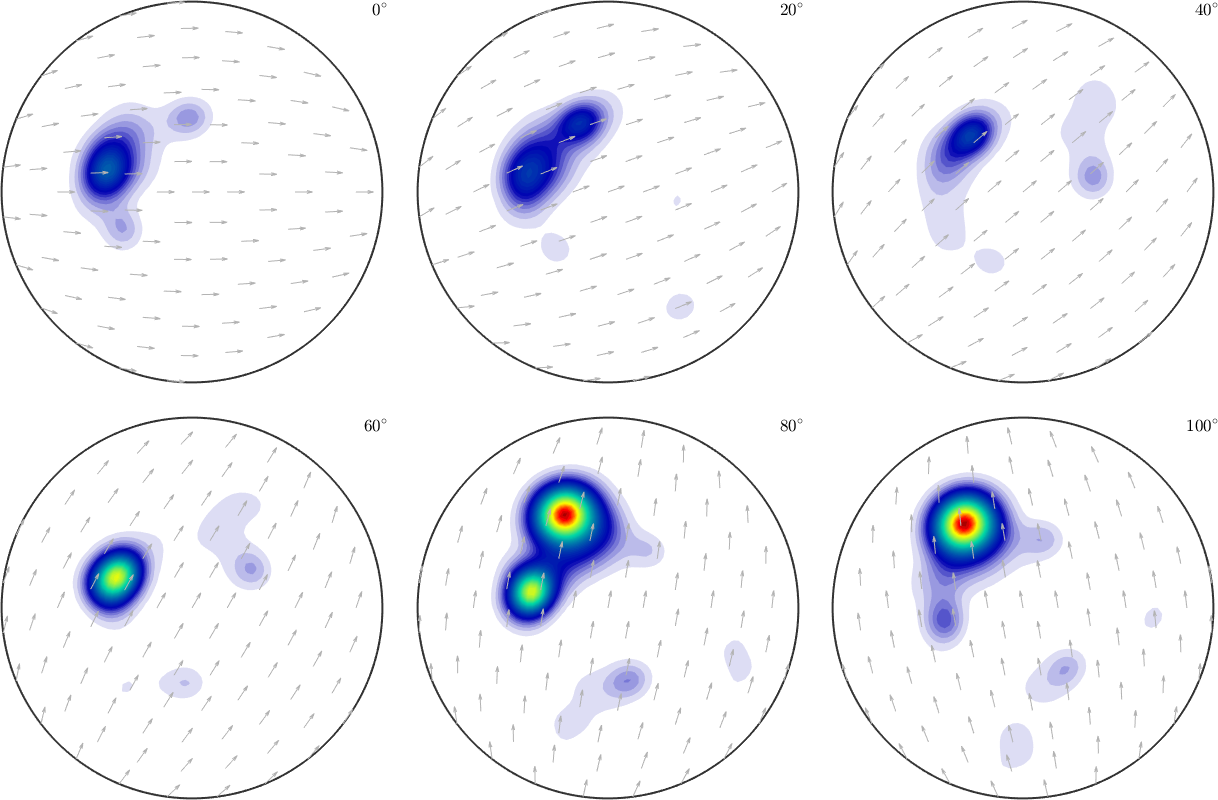
plot(SO3F1,'sigma')SO3F1 = SO3FunRBF (Quartz → y↑→x)
multimodal components
kernel: de la Vallee Poussin, halfwidth 5°
center: 19848 orientations, resolution: 5°
weight: 1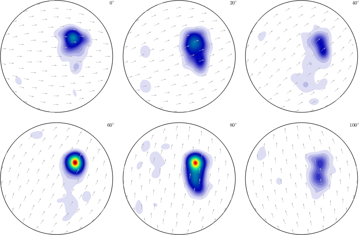
and an unimodal distributed ODF
R = orientation.byAxisAngle(vector3d.Y,pi/4,SO3F1.CS);
SO3F2 = SO3FunRBF(R,SO3DeLaValleePoussinKernel)

plot(SO3F2,'sigma')
SO3F2 = SO3FunRBF (Quartz → y↑→x)
unimodal component
kernel: de la Vallee Poussin, halfwidth 10°
center: 1 orientations
Bunge Euler angles in degree
phi1 Phi phi2 weight
90 45 270 1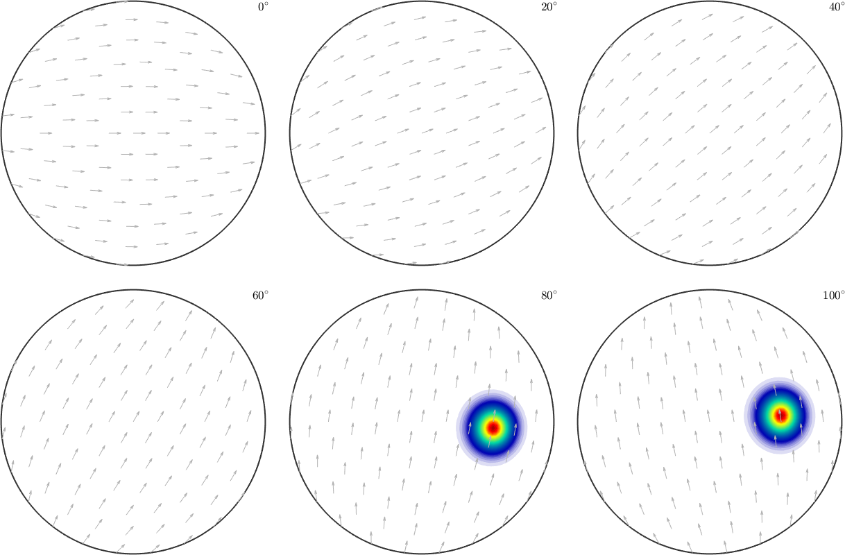
Basic arithmetic operations
Now the sum of these two rotational functions is again a rotational function, i.e., a function of type SO3Fun
1 + 2 * SO3F1 + SO3F2

plot(2 * SO3F1 + SO3F2,'sigma')
ans = SO3FunComposition (Quartz → y↑→x)
uniform component
weight: 1
multimodal components
kernel: de la Vallee Poussin, halfwidth 5°
center: 19848 orientations, resolution: 5°
weight: 2
unimodal component
kernel: de la Vallee Poussin, halfwidth 10°
center: 1 orientations
Bunge Euler angles in degree
phi1 Phi phi2 weight
90 45 270 1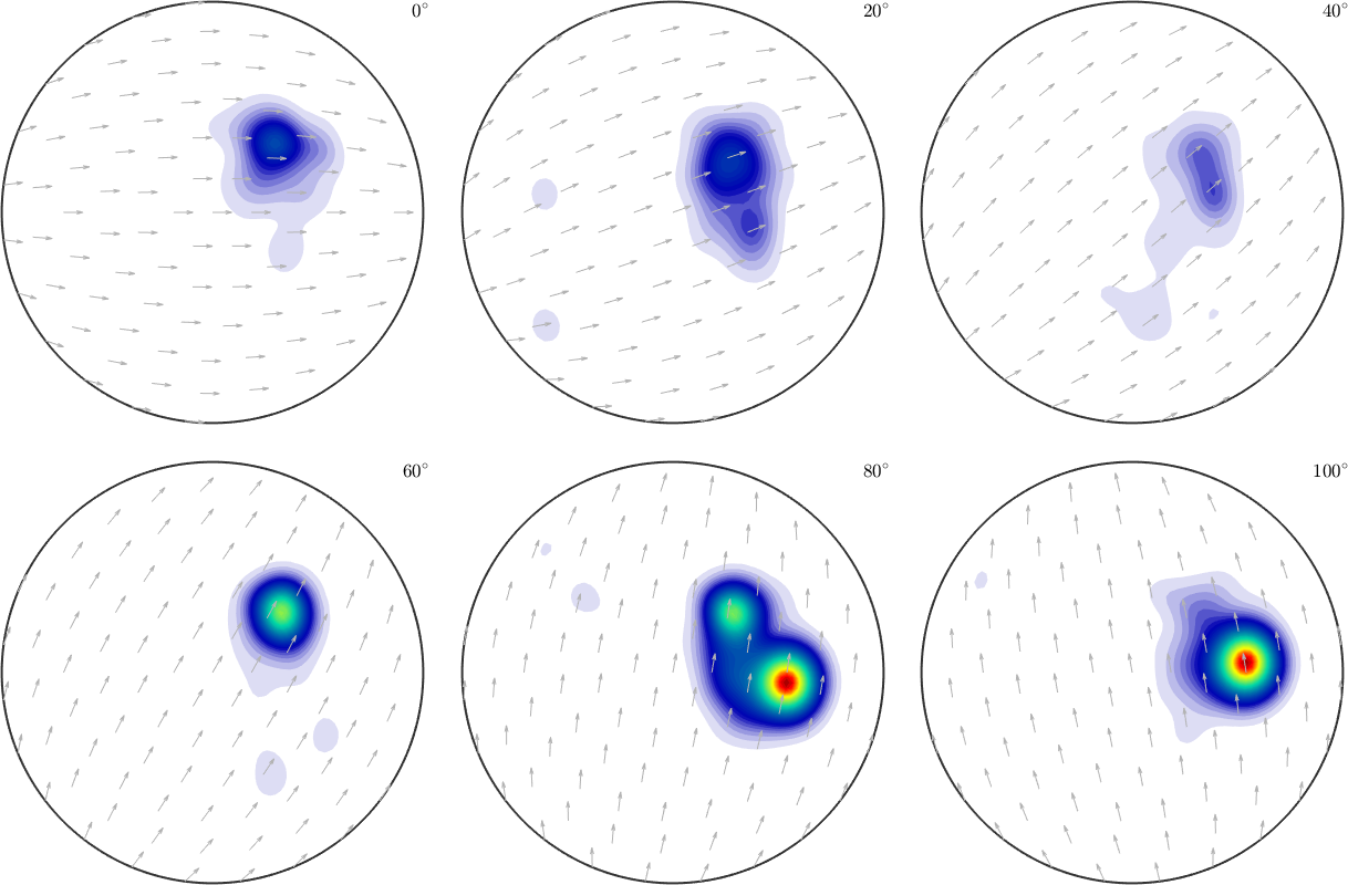
Accordingly, one can use all basic operations like -, *, ^, /, min, max, abs, sqrt to calculate with variables of type SO3Fun.
% the maximum between two functions
plot(max(2*SO3F1,SO3F2),'sigma');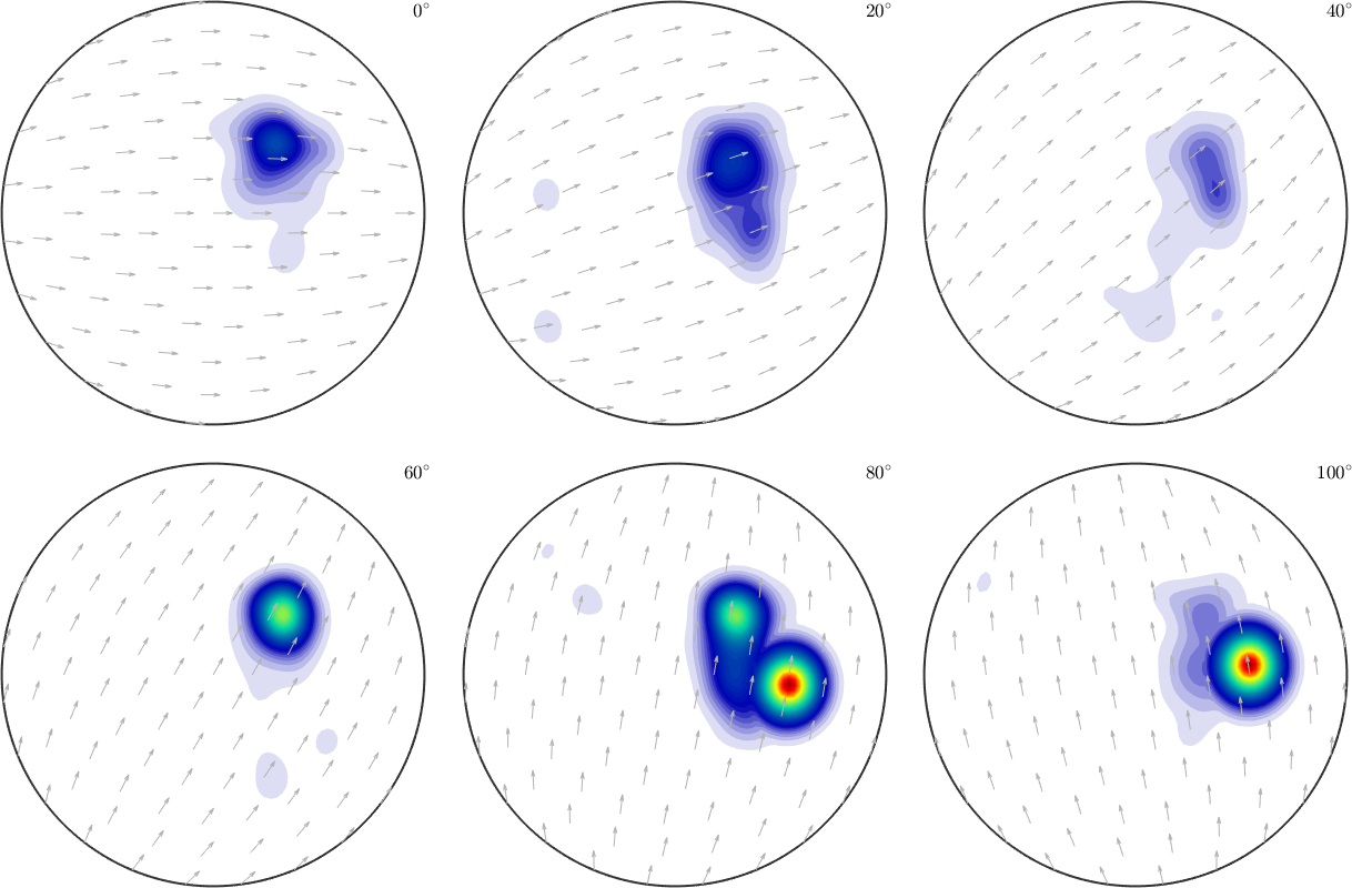
% the minimum between two functions
plot(min(2*SO3F1,SO3F2),'sigma');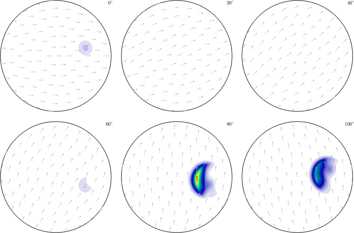
We also can work with the pointwise conj, exp or log of an SO3Fun.
For a given function \(f\colon SO(3) \to \mathbb C\) we get a second function \(g\colon SO(3) \to \mathbb C\) where \(g( {\bf R}) = f( {\bf R}^{-1})\) by the method inv, i.e.
g = inv(SO3F1)

SO3F1.eval(R)
g.eval(inv(R))
g = SO3FunRBF (y↑→x → Quartz)
multimodal components
kernel: de la Vallee Poussin, halfwidth 5°
center: 19848 orientations, resolution: 5°
weight: 1
ans =
2.3745
ans =
4.2858Local Extrema
The above mentioned functions min and max have very different use cases
- if a single rotational function is provided the global maximum / minimum of the function is computed
- if two rotational functions are provided, a rotational function defined as the pointwise min/max between these two functions is computed
- if a rotational function and a single number are passed as arguments a rotational function defined as the pointwise min/max between the function and the value is computed
- if additionally the option
'numLocal'is provided the certain number of local minima / maxima is computed
plot(2 * SO3F1 + SO3F2,'phi2',(0:3)*30*degree)

% compute and mark the global maximum
[maxValue, maxNodes] = max(2 * SO3F1 + SO3F2,'numLocal',2)
annotate(maxNodes)
maxValue =
260.27
212.31
maxNodes = orientation (Quartz → y↑→x)
size: 2 x 1
Bunge Euler angles in degree
phi1 Phi phi2
89.904 44.7846 270.085
133.047 34.5158 207.16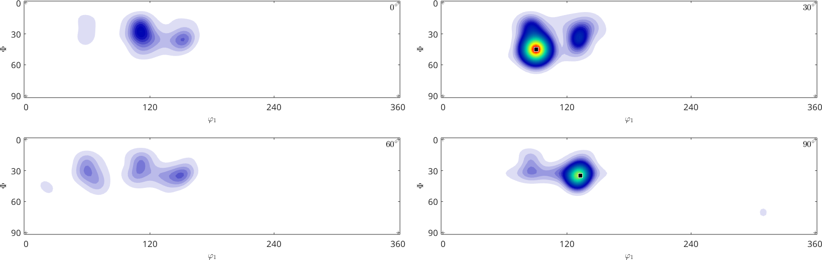
Integration
The surface integral of a spherical function can be computed by either mean or sum. The difference between both commands is that sum normalizes the integral of the identical function on the rotation group to \(8 \pi^2\), the command mean normalizes it to one. Compare
mean(SO3F1)

sum(SO3F1) / ( 8 * pi^2 )
ans =
1
ans =
1A practical application of integration is the computation of the \(L^2\)-norm which is defined for a \(SO(3)\) function \(f\) by
\[ \| f\|_2 = \left( \frac{1}{8\pi^2} \int_{SO(3)} \lvert f({\bf R}) \rvert^2 \,\mathrm d {\bf R} \right)^{1/2} \]
accordingly we can compute it by
sqrt(mean(abs(SO3F1).^2))ans =
3.7736or more efficiently by the command norm
norm(SO3F1)ans =
3.773Differentiation
The gradient of an \(SO(3)\) function in a specific point is described by a SO3TangentVector-object, which can be computed by the command grad
grad(SO3F1,R)ans = SO3TangentVector (y↑→x)
intern symmetries: Quartz → y↑→x
TagentSpace: leftVector
x y z
10.1343 -26.5867 -3.26427This SO3TangentVector describes an element of a tangent space on the rotation group \(SO(3)\) at some specific rotation.
For detailed information on this tangent space representation, see Tangent Space Representation on SO(3)
The gradients of a \(SO(3)\) function in all points form a \(SO(3)\) vector field and are returned by the function grad as a variable of type SO3VectorFieldHarmonic.
% compute the gradient as a vector field
G = grad(SO3F1)

% plot the gradient on top of the function
plot(SO3F1,'sigma')
hold on
plot(G,'color','black','linewidth',1,'resolution',5*degree)
hold off
G = SO3VectorFieldHarmonic (Quartz → y↑→x)
bandwidth: 48
tangent space: leftVector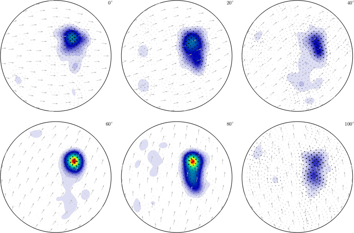
We observe long arrows at the positions of big changes in intensity and almost invisible arrows in regions of constant intensity.
Note that, roughly speaking, the gradient at a given rotation indicates the direction of steepest ascent of SO3F1. In the above plot, this gradient is represented by an arrow pointing along that direction. By following this arrow via the exponential map, one obtains a new rotation.
Rotating orientation dependent functions
Rotating an orientation dependent function works with the command rotate
% define a rotation
rot = rotation.byEuler(30*degree,0*degree,90*degree,'Bunge');

% rotate the ODF
SO3F = rotate(SO3FunHarmonic(2 * SO3F1 + SO3F2),rot)

% and plot it
plot(SO3F,'sigma')
SO3F = SO3FunHarmonic (Quartz → y↑→x)
bandwidth: 48
weight: 3