Colorbars
Unlike the common MATLAB command colorbar the MTEX command mtexColorbar allows you to add a colorbar to all subplots in a figure.
% this defines some model ODFs
cs = crystalSymmetry('-3m');

mod1 = orientation.byEuler(110*degree,30*degree,80*degree,cs);
mod2 = orientation.byEuler(310*degree,70*degree,40*degree,cs);
odf = 0.7*unimodalODF(mod1) + 0.3*unimodalODF(mod2);

% plot some pole figures
plotPDF(odf,Miller({1,0,0},{1,1,1},cs))

% and add a colorbar to each pole figure
mtexColorbar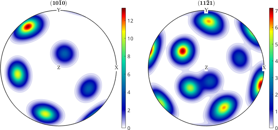
Executing the command mtexColorbar twice deletes the colorbar. You can also have a horizontal colorbar at the bottom of the figure by setting the option 'location' to 'southOutside'. Further, we can set a title to the colorbar to describe the unit.
% delete vertical colorbar
mtexColorbar

% add horizontal colorbars
mtexColorbar('location','southOutSide','title','mrd')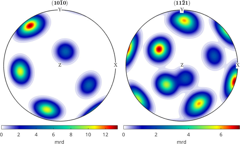
If color range is set to equal in an MTEX figure only one colorbar is added (see. Color Coding).
mtexColorbar       % delete colorbar
setColorRange('equal'); % set equal color range to all plots
mtexColorbar       % create a new colorbar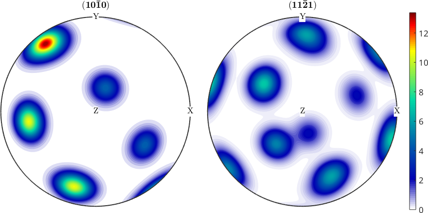
Annotating Directions, Orientations, Fibers
Pole figures or inverse pole figures are much better readable if they include specimen or crystal directions. Using the MTEX command annotate one can easily add specimen coordinate axes to a pole figure plot.
annotate(vector3d(1,1,1),'label',{'(111)'},'BackgroundColor','w')
The command annotate allows also to mark crystal directions in inverse pole figures.
plotIPDF(odf,[xvector,zvector],'antipodal','marginx',10)
mtexColorMap white2black

annotate(Miller({2,-1,-1,0},{2,-1,-1,1},cs), ...
  'all','labeled','BackgroundColor','yellow')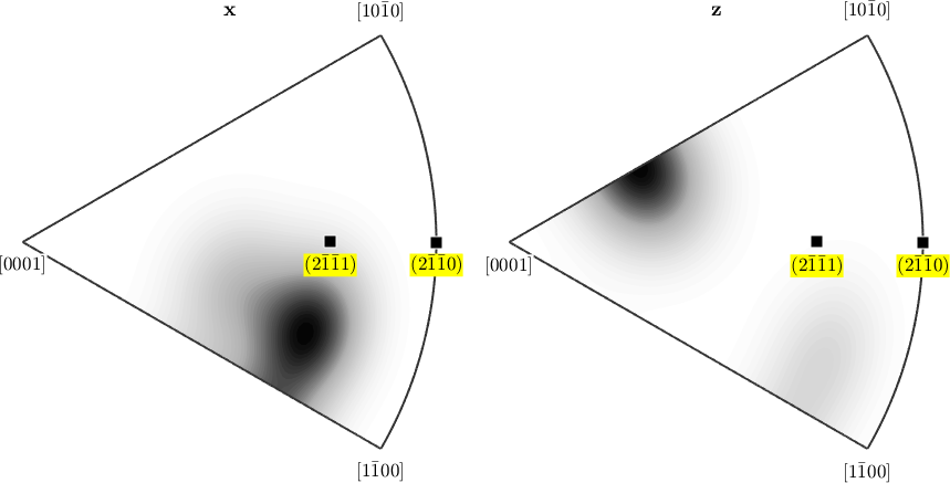
One can also mark specific orientations in pole figures or in inverse pole figures.
plotIPDF(odf,[xvector,zvector],'antipodal')
mtexColorMap white2black
annotate(mod1,...
    'marker','s','MarkerSize',6,'MarkerFaceColor','r',...
    'label','A','color','w')

annotate(mod2,...
    'marker','s','MarkerSize',6,'MarkerFaceColor','g',...
    'label','B')

drawNow(gcm,'figSize','normal')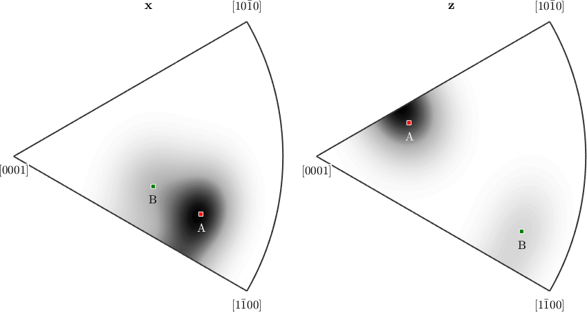
as well as in ODF plots
plot(odf,'sigma')
mtexColorMap white2black
annotate(mod1,'label','A','textColor','r',...
    'MarkerSize',15,'MarkerEdgeColor','r','MarkerFaceColor','none')

annotate(mod2,'label','B','textColor','b',...
  'MarkerSize',15,'MarkerEdgeColor','b','MarkerFaceColor','none')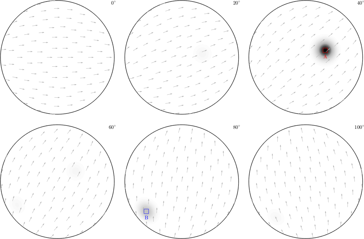
or orientation scatter plots
ori = odf.discreteSample(200);
scatter(ori);
annotate(mod1,...
  'MarkerSize',10,'MarkerEdgeColor','r','MarkerFaceColor','r')
annotate(mod2,...
  'MarkerSize',10,'MarkerEdgeColor','g','MarkerFaceColor','g')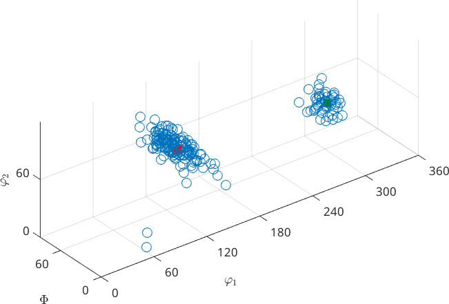
Legends
If you have multiple data in one plot then it makes sense to add a legend saying which color / symbol correspond to which data set. The key is to use the option 'DisplayName' available for all plotting commands to include the resulting graphical object into the legend and give it a name.
plotPDF(odf,Miller({1,0,0},{1,1,1},cs))
plot(ori,'MarkerFaceColor','k','MarkerEdgeColor','black','add2all',...
  'DisplayName','randomSample')

f = fibre(Miller({1,1,-2,1},cs),vector3d.Y);
plot(f,'color','red','linewidth',2,'add2all','DisplayName','fibre')

legend show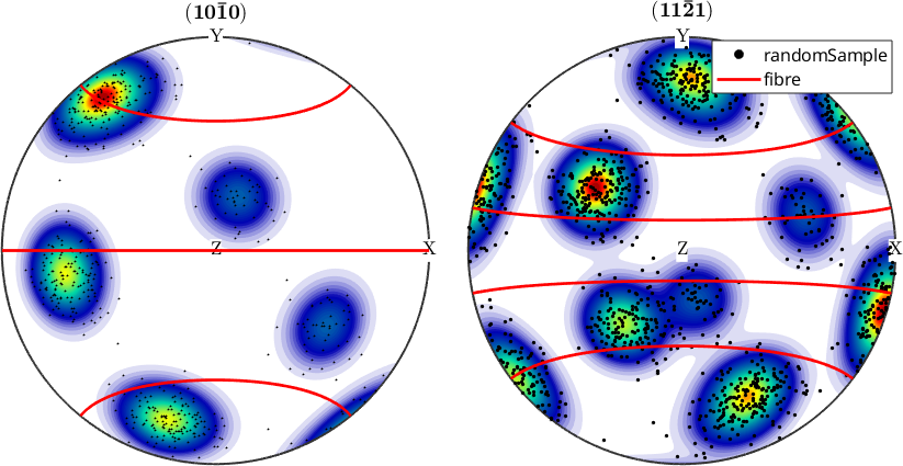
The following example compares the Fourier coefficients of the fibre ODF with the Fourier coefficients of an unimodal ODF.
close all
plotSpektra(FourierODF(odf,32),'DisplayName','Unimodal ODF')
hold on
fodf = fibreODF(Miller(1,0,0,cs),zvector);
plotSpektra(FourierODF(fodf,32),'DisplayName','Fibre ODF');
hold off
legend show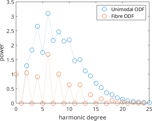
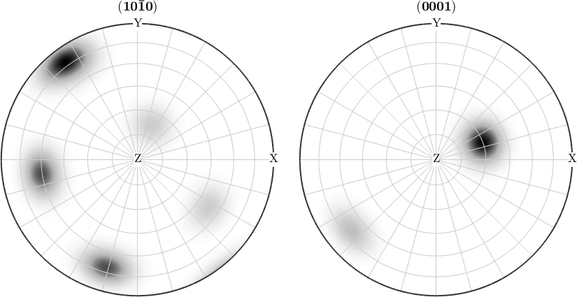
Adding a Spherical Grid
Sometimes it is useful to have a spherical grid in your plot to make the projection easier to understand or if you need to know some angular relationships. For this reason, there is the option 'grid', which enables the grid and the option 'grid_res', which allows to specify the spacing of the grid lines.
plotPDF(odf,[Miller(1,0,0,cs),Miller(0,0,1,cs)],'grid','grid_res',15*degree,'antipodal');
mtexColorMap white2black