Transformation Texture edit page

Transformation Texture

During phase transformation or twinning the orientation of a crystal rapidly flips from an initial state oriA into a transformed state oriB. This relationship between the initial and transformed state can be described by an orientation relationship OR. To make the situation more precise, we consider the phase transformation from austenite to ferrite via the Nishiyama Wassermann orientation relationship

% parent and child crystal symmetry
csP = crystalSymmetry('432','mineral','Austenite');
csC = crystalSymmetry('432','mineral','Ferrite');

% the orientation relationship
p2c = orientation.NishiyamaWassermann(csP,csC);

Now an arbitrary Austenite orientation

oriA = orientation.rand(csP)

oriA = orientation (Austenite → xyz)
 
  Bunge Euler angles in degree
     phi1     Phi    phi2
  238.265 100.111 261.631

is transformed in one of the following Ferrite orientations

oriB = variants(p2c,oriA)

oriB = orientation (Ferrite → xyz)
  size: 1 x 12
 
  Bunge Euler angles in degree
     phi1     Phi    phi2
  103.932 86.7036  358.69
  355.703 138.501 117.565
  32.9982 39.0212 296.271
  309.435 56.6843 289.021
  196.065 81.8242 166.834
  64.9644 34.3738  90.382
  191.632 100.789 346.732
  76.7717 122.155 106.235
  145.575 36.0662  266.16
  53.6238 125.498 273.221
  332.836 52.5099 95.3293
  104.406 67.2378 178.582

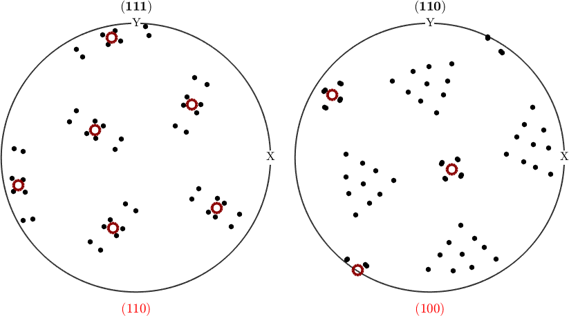
These 12 Ferrite orientations are called variants of the orientation relationship. Lets visualize them in a pole figure plot

hC = Miller({1,1,1},{1,1,0},csC);
hP = Miller({1,1,0},{1,0,0},csP);

% plot the child variants
plotPDF(oriB,hC,'MarkerSize',5,'markerColor','black','figSize','medium');

% and on top the parent orientation
opt = {'MarkerFaceColor','none','MarkerEdgeColor','darkred','linewidth',3};
for k = 1:2
  nextAxis(k)
  hold on
  plot(oriA * hP(k).symmetrise ,opt{:})
  xlabel(char(hP(k),'latex'),'Color','red','Interpreter','latex')
  hold off
end
drawNow(gcm)

In case we have multiple parent orientations following some initial orientation distribution function odf

% define a model ODF
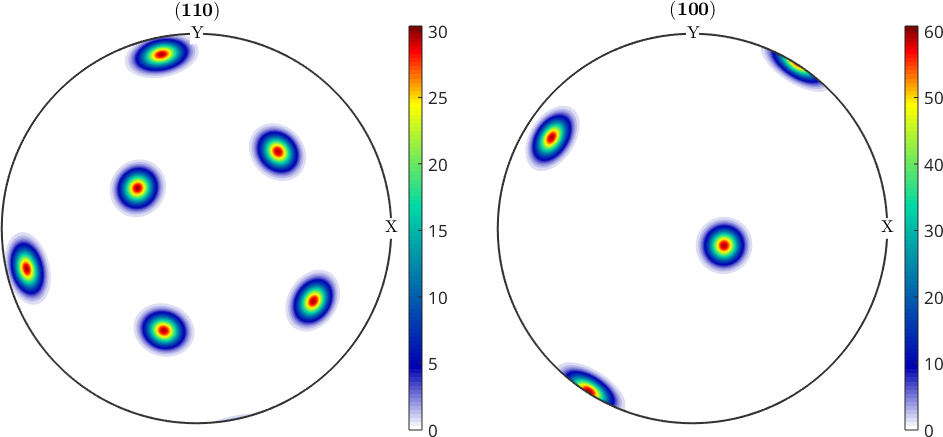
odfA = unimodalODF(oriA,'halfwidth',5*degree)

plotPDF(odfA,hP,'figSize','medium')
mtexColorbar

odfA = SO3FunRBF (Austenite → xyz)
 
  unimodal component
  kernel: de la Vallee Poussin, halfwidth 5°
  center: 1 orientations
 
  Bunge Euler angles in degree
     phi1     Phi    phi2  weight
  238.265 100.111 261.631       1

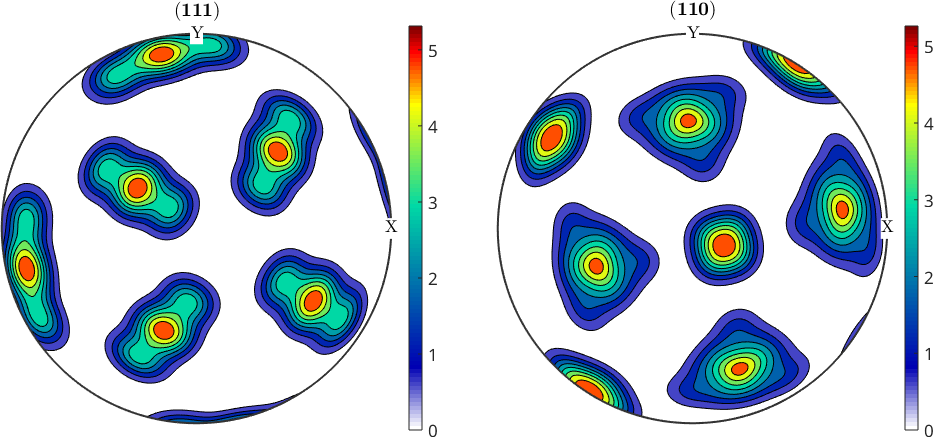
We can draw some random orientations according this model ODF and apply the same commands variants to compute all transformed orientations in one step

% number of discrete orientations
n = 10000;
oriASim = odfA.discreteSample(n)

% transform the orientations
oriBSim = variants(p2c,oriASim)

% show the result
plotPDF(oriBSim,hC,'contourf','figSize','medium');
mtexColorbar

oriASim = orientation (Austenite → xyz)
  size: 10000 x 1
 
oriBSim = orientation (Ferrite → xyz)
  size: 10000 x 12

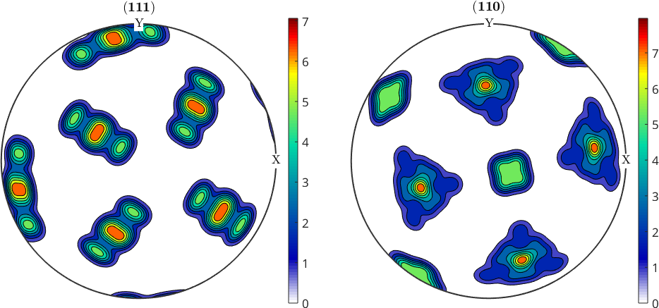
An alternative and better approach is to directly use odfA as an input to the function variants. In this case the output is the orientation distribution function of the transformed material

% compute the child ODF
odfB = variants(p2c,odfA)

% plot
plotPDF(odfB,hC,'contourf','figSize','medium');
mtexColorbar

odfB = SO3FunHarmonic (Ferrite → xyz)
  bandwidth: 48
  weight: 1

We observe that the transformed ODF computed by the latter approach is sharper and shows more details when compared with the ODF computed from discrete orientations. We may quantify this difference by computing the texture index of both ODFs

% texture index of the transformed ODF computed from discrete orientations
odfBSim = calcDensity(oriBSim)
norm(odfBSim)^2

odfBSim = SO3FunHarmonic (Ferrite → xyz)
  bandwidth: 25
  weight: 1
 
ans =
    3.4766

% texture index of the directly computed transformed ODF
norm(odfB)^2

ans =
   17.4509