Here we describe how to detect sample symmetry in an arbitrarily rotated ODF.
A synthetic example
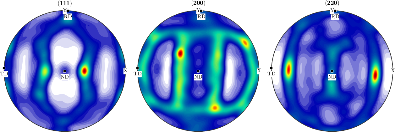
We start by modeling a orthotropic ODF with cubic crystal symmetry.
CS = crystalSymmetry('cubic');
SS = specimenSymmetry('222');

% some component center
ori = [orientation.byEuler(135*degree,45*degree,120*degree,CS,SS) ...
  orientation.byEuler( 60*degree, 54.73*degree, 45*degree,CS,SS) ...
  orientation.byEuler(70*degree,90*degree,45*degree,CS,SS)...
  orientation.byEuler(0*degree,0*degree,0*degree,CS,SS)];

% with corresponding weights
c = [.4,.13,.4,.07];

% the model odf
odf = unimodalODF(ori(:),'weights',c,'halfwidth',12*degree)

% lets plot some pole figures
h = [Miller(1,1,1,CS),Miller(2,0,0,CS),Miller(2,2,0,CS)];
plotPDF(odf,h,'antipodal','silent','complete')
odf = SO3FunRBF (m-3m → y↑→x (222))
multimodal components
kernel: de la Vallee Poussin, halfwidth 12°
center: 4 orientations
Bunge Euler angles in degree
phi1 Phi phi2 weight
135 45 120 0.4
60 54.73 45 0.13
70 90 45 0.4
0 0 0 0.07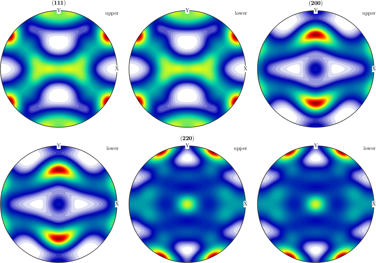
Reconstruct an ODF from simulated EBSD data
Next we simulated some EBSD data, rotate them and estimate an ODF from the individual orientations.
% define a sample rotation
rot = rotation.byEuler(15*degree,12*degree,-5*degree);


% Simulate individual orientations and rotate them.
% Note that we loose the sample symmetry by rotating the orientations
ori = rot * discreteSample(odf,1000)

% estimate an ODF from the individual orientations
odf_est = calcDensity(ori,'halfwidth',10*degree)

% and visualize it
plotPDF(odf_est,h,'antipodal',8,'silent');
ori = orientation (m-3m → y↑→x (222))
size: 1 x 1000
odf_est = SO3FunHarmonic (m-3m → y↑→x (222))
bandwidth: 25
weight: 1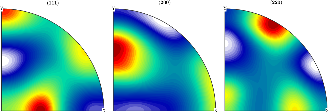
Detect the sample symmetry axis in the reconstructed ODF
We observe that the reconstructed ODF has almost orthotropic symmetry, but with respect to axes different from x, y, z. With the command centerSpecimen we can determine an rotation such that the rotated ODF has almost orthotropic symmetry with respect to x, y, z. The second argument is some starting direction where MTEX looks for a symmetry axis.
[odf_corrected,rot_inv] = centerSpecimen(odf_est);

plotPDF(odf_corrected,h,'antipodal',8,'silent')

% the difference between the applied rotation and the estimate rotation
angle(rot,inv(rot_inv)) / degree
ans =
15.6088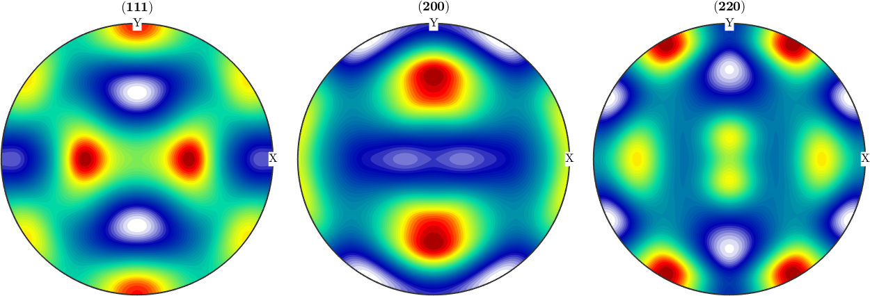
Sample symmetry in an ODF computed from pole figure data
In the next example we apply the function centerSpecimen to an ODF estimated from pole figure data. Lets start by importing them
fname = fullfile(mtexDataPath,'PoleFigure','aachen_exp.EXP');
pf = PoleFigure.load(fname);

plot(pf,'silent')
In a second step we compute an ODF from the pole figure data
odf = calcODF(pf,'silent')

plotPDF(odf,h,'antipodal','silent')
odf = SO3FunRBF (m-3m → y↑→x)
multimodal components
kernel: de la Vallee Poussin, halfwidth 5°
center: 4958 orientations, resolution: 5°
weight: 1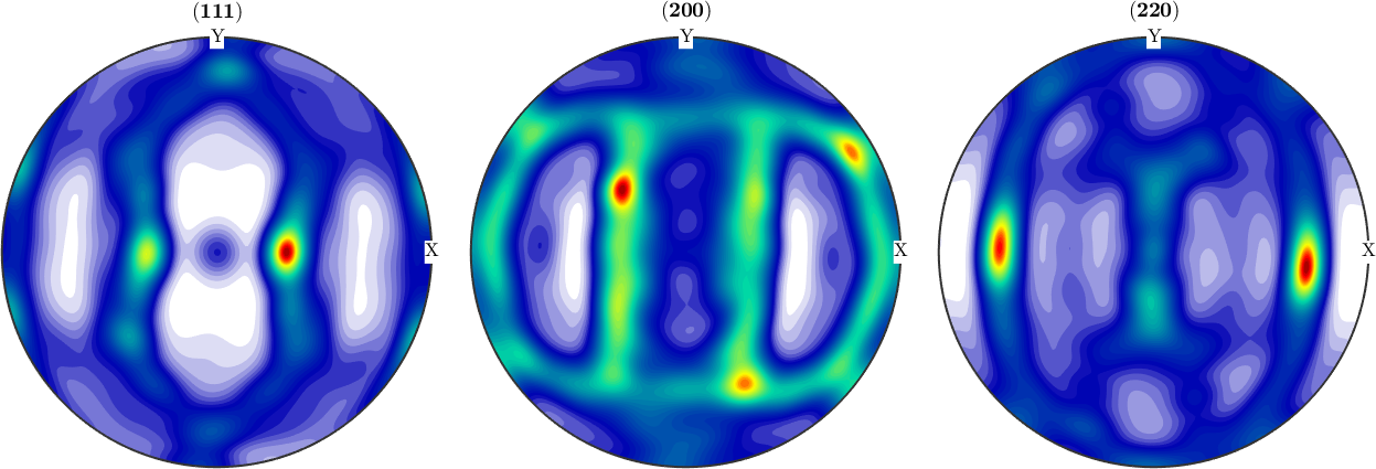
Finally, we detect the orthotropic symmetry axes a1, a2, a3 by
[~,~,a1,a2] = centerSpecimen(odf,yvector,'Fourier')
a3 = cross(a1,a2)

annotate([a1,a2,a3],'label',{'RD','TD','ND'},'backgroundcolor','w','MarkerSize',8)
a1 = vector3d (y↑→x)
x y z
0.0499876 0.998745 0.00325886
a2 = vector3d (y↑→x)
x y z
-0.99875 0.0499879 0
a3 = vector3d (y↑→x)
x y z
-0.000162903 -0.00325478 0.999995