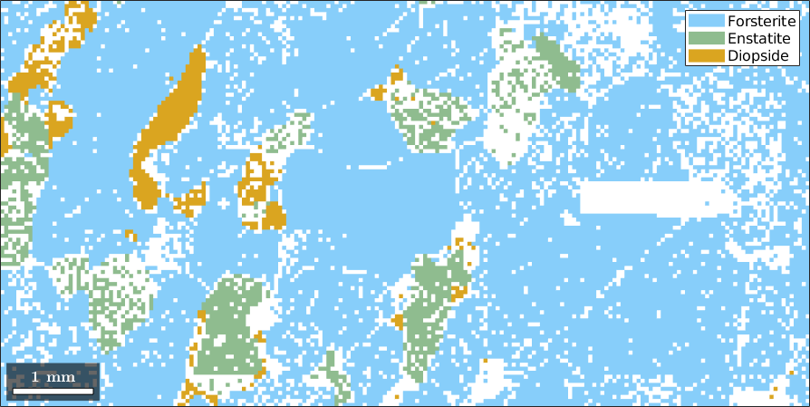
In this section we discuss how to select specific EBSD data by certain properties. Let us first import some example EBSD data using the command mtexdata.
mtexdata forsteriteebsd = EBSD (y↑→x)
Phase Orientations Mineral Color Symmetry Crystal reference frame
0 58485 (24%) notIndexed
1 152345 (62%) Forsterite LightSkyBlue mmm
2 26058 (11%) Enstatite DarkSeaGreen mmm
3 9064 (3.7%) Diopside Goldenrod 12/m1 X||a*, Y||b*, Z||c
Properties: bands, bc, bs, error, mad
Scan unit : um
X x Y x Z : [0, 36550] x [0, 16750] x [0, 0]
Normal vector: (0,0,1)These data consist of three indexed phases, Forsterite, Enstatite and Diopside. The not indexed phase called not Indexed. The phases can be visualized by
close all;
plot(ebsd)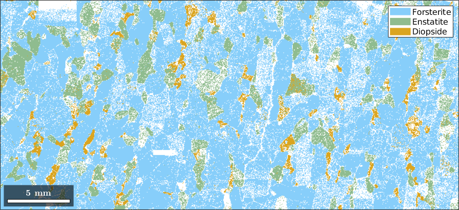
Selecting a certain phase
After import the EBSD data are stored in the variable ebsd which is essentially a long list of x and y values together with phase information and orientations. In order to restrict this list to a certain phase just use the mineral name as an index, i.e.
ebsd('Forsterite')ans = EBSD (y↑→x)
Phase Orientations Mineral Color Symmetry Crystal reference frame
1 152345 (100%) Forsterite LightSkyBlue mmm
Properties: bands, bc, bs, error, mad
Scan unit : um
X x Y x Z : [0, 36550] x [0, 16750] x [0, 0]
Normal vector: (0,0,1)contains only the Forsterite measurements. In order to extract a couple of phases, the mineral names have to be grouped in curled parenthesis.
ebsd({'Fo','En'})ans = EBSD (y↑→x)
Phase Orientations Mineral Color Symmetry Crystal reference frame
1 152345 (85%) Forsterite LightSkyBlue mmm
2 26058 (15%) Enstatite DarkSeaGreen mmm
Properties: bands, bc, bs, error, mad
Scan unit : um
X x Y x Z : [0, 36550] x [0, 16750] x [0, 0]
Normal vector: (0,0,1)As an example, let us plot the Forsterite data.
close all
plot(ebsd('Forsterite'),ebsd('Forsterite').orientations)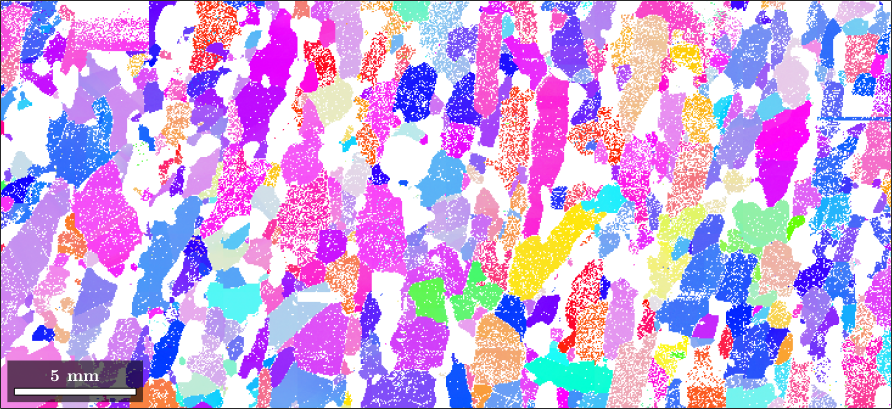
The data is colorized according to its orientation. By default color of an orientation is determined by its position in the 001 inverse pole figure which itself is colored as
ipfKey = ipfColorKey(ebsd('Forsterite'));
plot(ipfKey)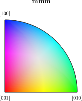
Restricting to a region of interest
If one is not interested in the whole data set but only in those measurements inside a certain polygon, the restriction can be constructed as follows:
First define a region by [xmin ymin xmax-xmin ymax-ymin]
region = [5 2 10 5]*10^3;plot the ebsd data together with the region of interest
close all
plot(ebsd)
rectangle('position',region,'edgecolor','r','linewidth',2)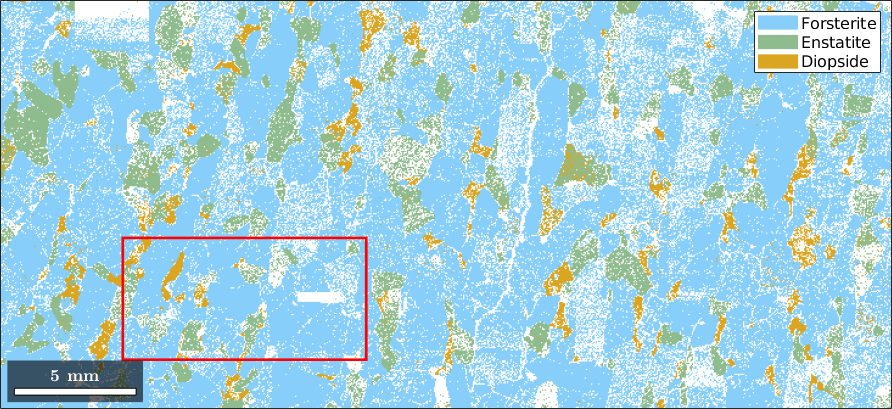
The command inpolygon checks for each EBSD data point whether it is inside a polygon or not, i.e.
condition = inpolygon(ebsd,region);results in a large vector of TRUE and FALSE stating which data points are inside the region. Restricting the EBSD data by this condition is done via
ebsd = ebsd(condition)ebsd = EBSD (y↑→x)
Phase Orientations Mineral Color Symmetry Crystal reference frame
0 4052 (20%) notIndexed
1 14093 (69%) Forsterite LightSkyBlue mmm
2 1397 (6.9%) Enstatite DarkSeaGreen mmm
3 759 (3.7%) Diopside Goldenrod 12/m1 X||a*, Y||b*, Z||c
Properties: bands, bc, bs, error, mad
Scan unit : um
X x Y x Z : [5000, 15000] x [2000, 7000] x [0, 0]
Normal vector: (0,0,1)plot
close all
plot(ebsd)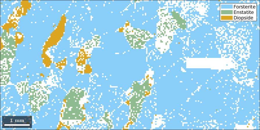
Note, that you can also select a polygon by mouse using the command
poly = selectPolygonRemove Inaccurate Orientation Measurements
Most EBSD measurements contain quantities indicating inaccurate measurements, e.g. MAD (mean angular deviation) in the case of Oxford Channel programs, or CI (Confidence Index) in the case of OIM-TSL programs.
close all
plot(ebsd,ebsd.mad)
mtexColorbar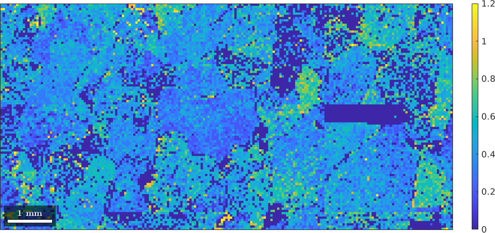
or
close all
plot(ebsd,ebsd.bc)
mtexColorbar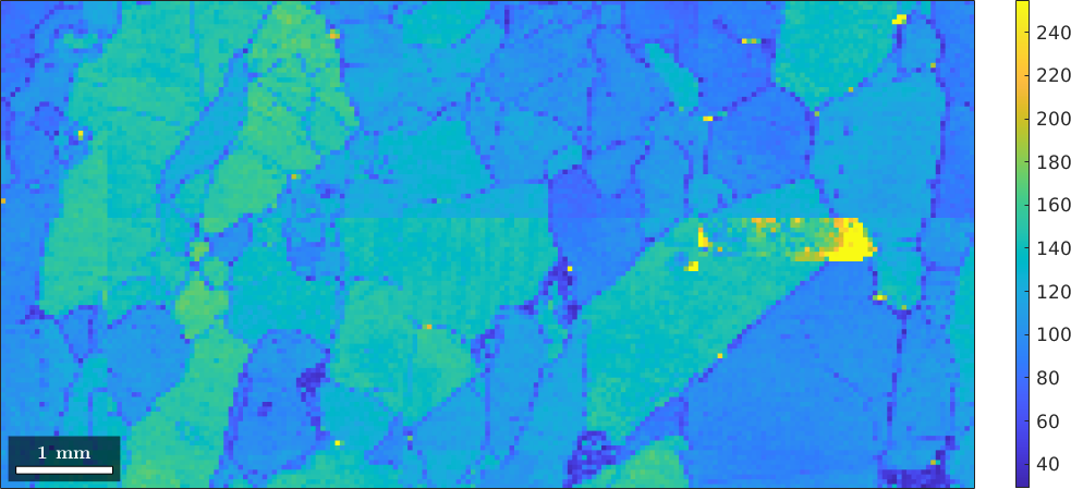
Here we will use the MAD to identify and eliminate inaccurate measurements.
% plot a histogram
close all
histogram(ebsd.mad)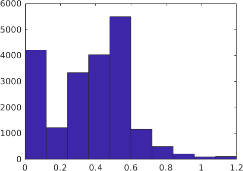
% take only those measurements with MAD smaller then one
ebsd_corrected = ebsd(ebsd.mad<0.8)
ebsd_corrected = EBSD (y↑→x)
Phase Orientations Mineral Color Symmetry Crystal reference frame
0 4052 (21%) notIndexed
1 13359 (69%) Forsterite LightSkyBlue mmm
2 1333 (6.9%) Enstatite DarkSeaGreen mmm
3 676 (3.5%) Diopside Goldenrod 12/m1 X||a*, Y||b*, Z||c
Properties: bands, bc, bs, error, mad
Scan unit : um
X x Y x Z : [5000, 15000] x [2000, 7000] x [0, 0]
Normal vector: (0,0,1)close all
plot(ebsd_corrected)