Functions on the circle are periodic functions. Hence they may be represented as weighted sums of sines and cosines (Fourier series). A spherical function \(f\) can be written as series of the form
\[ f(x) = \sum_{k=-N}^N \hat f_k e^{-ikx} \]
with respect to Fourier coefficients \(\hat f_k\). Note that \(f\) is \(2\pi\)-periodic.
Within the class S1FunHarmonic spherical functions are represented by their Fourier coefficients which are stored in the field fun.fhat. As an example lets define a Fourier series which Fourier coefficients \(\hat f_0 = 1\), \(\hat f_1 = 0\), \(\hat f_{-1} = 3\), \(\hat f_2 = 4\) and \(\hat f_{-2} = 0\)
fun = S1FunHarmonic([0;3;1;0;4])

clf
plot(fun)
fun = S1FunHarmonic
bandwidth: 2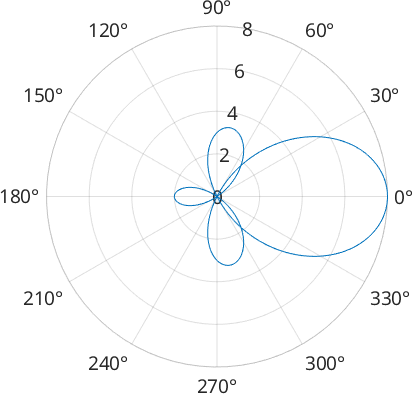
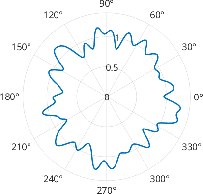
More practically, periodic functions appear after density estimation from circular data, e.g. of the azimuth angle of three dimensional vectors
% some random directions
v = vector3d.rand(1000);

% perform density estimation of the azimuth angle
fun = calcDensity(v.rho,'periodic')

clf
plot(fun,'linewidth',2)
fun = S1FunHarmonic
bandwidth: 61
isReal: true