Basics of the plot types for individual orientations data
This section gives an overview over the possibilities that MTEX offers to visualize orientation data. Let us first load a sample EBSD data set
mtexdata forsteriteebsd = EBSD (y↑→x)
Phase Orientations Mineral Color Symmetry Crystal reference frame
0 58485 (24%) notIndexed
1 152345 (62%) Forsterite LightSkyBlue mmm
2 26058 (11%) Enstatite DarkSeaGreen mmm
3 9064 (3.7%) Diopside Goldenrod 12/m1 X||a*, Y||b*, Z||c
Properties: bands, bc, bs, error, mad
Scan unit : um
X x Y x Z : [0, 36550] x [0, 16750] x [0, 0]
Normal vector: (0,0,1)and select all individual orientations of the Iron phase
ebsd('Fo').orientationsans = orientation (Forsterite → y↑→x)
size: 152345 x 1Scatter Pole Figure Plot
A pole figure showing scattered points of these data figure can be produced by the command plotPDF.
plotPDF(ebsd('Fo').orientations,Miller(1,0,0,ebsd('Fo').CS))I'm plotting 1250 random orientations out of 152345 given orientations
You can specify the the number points by the option "points".
The option "all" ensures that all data are plotted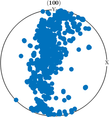
Scatter (Inverse) Pole Figure Plot
Accordingly, scatter points in inverse pole figures are produced by the command plotIPDF.
plotIPDF(ebsd('Fo').orientations,xvector)I'm plotting 12500 random orientations out of 152345 given orientations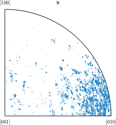
Scatter Plot in ODF Sections
The plotting of scatter points in sections of the orientation space is carried out by the command plotSection. In the above examples, the number of plotted orientations was chosen automatically such that the plots not to become too crowded with points. The number of randomly chosen orientations can be specified by the option 'points'.
plotSection(ebsd('Fo').orientations,'points',1000,'sigma','sections',9)plotting 1000 random orientations out of 152345 given orientations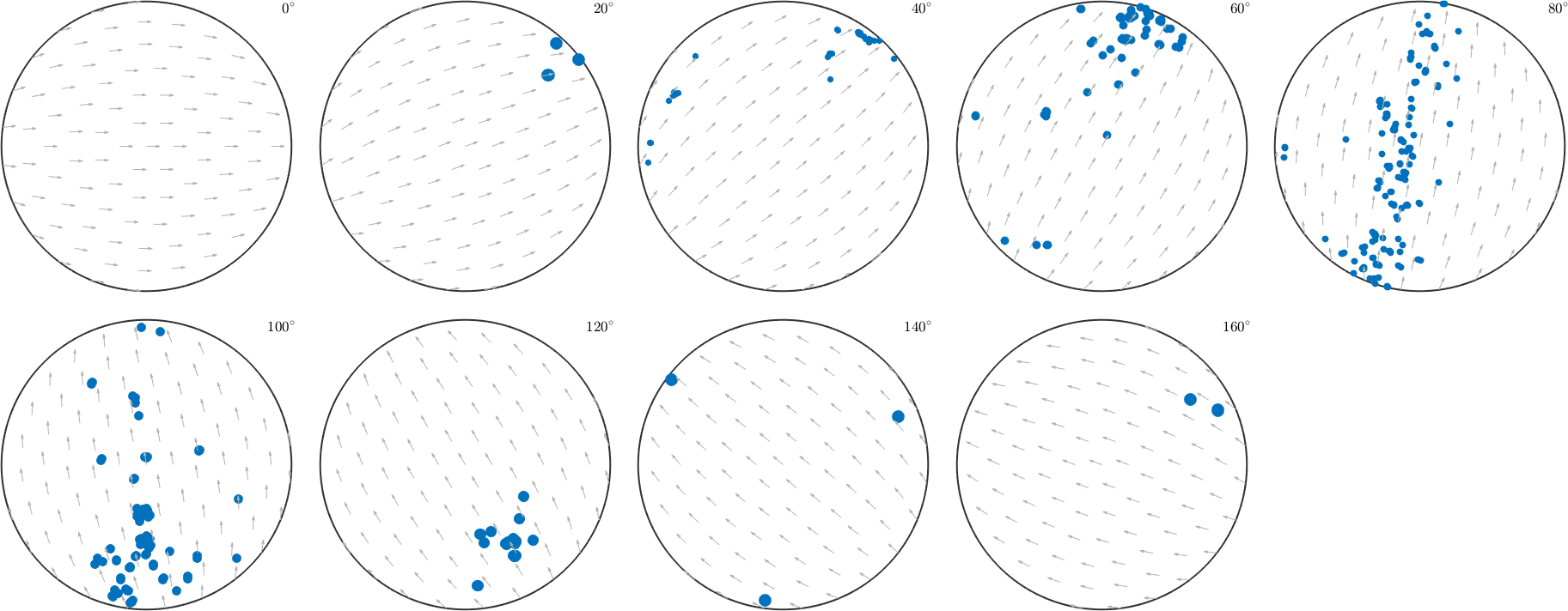
Scatter Plot in Axis Angle or Rodrigues Space
Another possibility is to plot the single orientations directly into the orientation space, i.e., either in axis/angle parametrization or in Rodrigues parametrization.
scatter(ebsd('Fo').orientations)plot 2000 random orientations out of 152345 given orientations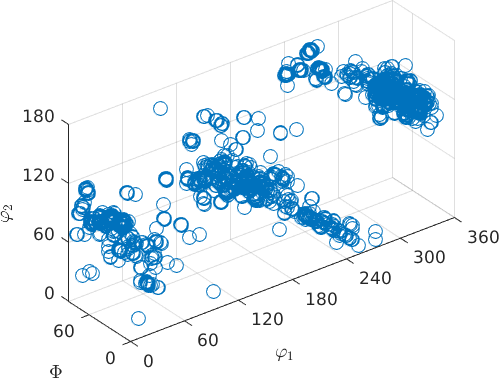
Here, the optional option 'center' specifies the center of the unique region in the orientation space.
Orientation plots for EBSD and grains
Since EBSD and grain data involves single orientations, the above plotting commands are also applicable for those objects.
Let us consider some grains reconstructed from the EBSD data
grains = calcGrains(ebsd);Then the scatter plot of the individual orientations of the Iron phase in the inverse pole figure is achieved by
plotIPDF(ebsd('Fo').orientations,xvector,'points',1000, 'MarkerSize',3);I'm plotting 1000 random orientations out of 152345 given orientations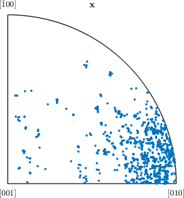
In the same way, the mean orientations of grains can be visualized
hold on
plotIPDF(grains('Fo').meanOrientation,xvector,'points',500, 'MarkerSize',3);
hold off
I'm plotting 500 random orientations out of 4092 given orientations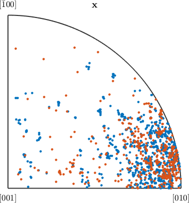
One can also use different colors on the scatter points
h = [Miller(1,0,0,ebsd('Fo').CS),Miller(1,1,0,ebsd('Fo').CS)];
plotPDF(ebsd('Fo').orientations,ebsd('Fo').mad,h,'antipodal','MarkerSize',4)
I'm plotting 1250 random orientations out of 152345 given orientations
You can specify the the number points by the option "points".
The option "all" ensures that all data are plotted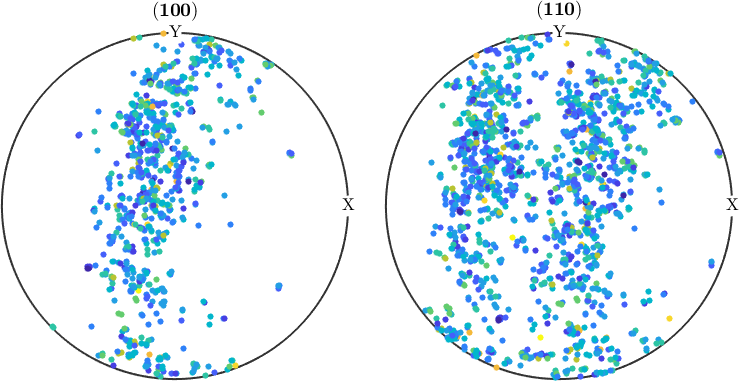
or some arbitrary data vector
plotSection(grains('Fo').meanOrientation,log(grains('Fo').area),...
  'sigma','sections',9,'MarkerSize',10);
plotting 2000 random orientations out of 4092 given orientations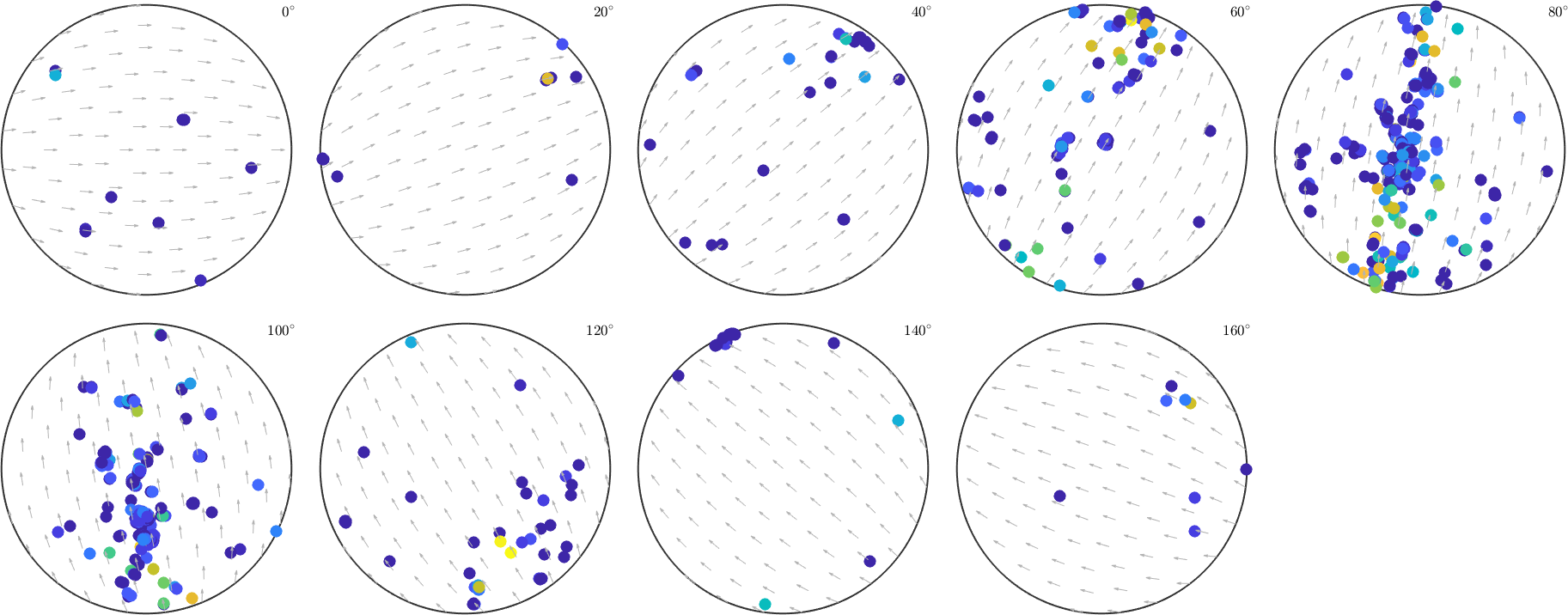
See also Scatter plots for more information about scatter plot and projections for more information on spherical projections.