TODO
Import an Elasticity Tensor
Let us start by importing the elastic stiffness tensor of an Olivine crystal in reference orientation from a file.
fname = fullfile(mtexDataPath,'tensor','Olivine1997PC.GPa');

cs = crystalSymmetry('mmm',[4.7646 10.2296 5.9942],'mineral','Olivin');

C = stiffnessTensor.load(fname,cs)
C = stiffnessTensor (Olivin)
unit: GPa
rank: 4 (3 x 3 x 3 x 3)
tensor in Voigt matrix representation:
320.5 68.2 71.6 0 0 0
68.2 196.5 76.8 0 0 0
71.6 76.8 233.5 0 0 0
0 0 0 64 0 0
0 0 0 0 77 0
0 0 0 0 0 78.7Christoffel Tensor
The Christoffel Tensor is symmetric because of the symmetry of the elastic constants. The eigenvalues of the 3x3 Christoffel tensor are three positive values of the wave moduli which corresponds to \rho Vp^2 , \rho Vs1^2 and \rho Vs2^2 of the plane waves propagating in the direction n. The three eigenvectors of this tensor are then the polarization directions of the three waves. Because the Christoffel tensor is symmetric, the polarization vectors are perpendicular to each other.
% It is computed for a specific direction x by the
% command <tensor.ChristoffelTensor.html ChristoffelTensor>.

T = ChristoffelTensor(C,vector3d.X)
T = ChristoffelTensor (Olivin)
rank: 2 (3 x 3)
320.5 0 0
0 78.7 0
0 0 77Elastic Wave Velocity
The Christoffel tensor is the basis for computing the direction dependent wave velocities of the p, s1, and s2 wave, as well as of the polarization directions. Therefore, we need also the density of the material, e.g.,
rho = 3.355rho =
3.355which we can write directly into the elastic stiffness tensor
C = addOption(C,'density',rho)C = stiffnessTensor (Olivin)
unit : GPa
density: 3.355
rank : 4 (3 x 3 x 3 x 3)
tensor in Voigt matrix representation:
320.5 68.2 71.6 0 0 0
68.2 196.5 76.8 0 0 0
71.6 76.8 233.5 0 0 0
0 0 0 64 0 0
0 0 0 0 77 0
0 0 0 0 0 78.7the single crystal wave velocities are now computed by the command stiffnessTensor.velocity.html velocity>
[vp,vs1,vs2,pp,ps1,ps2] = velocity(C)vp = S2FunTri (y↑→x)
vertices: 18338 x 1
vs1 = S2FunTri (y↑→x)
vertices: 18338 x 1
vs2 = S2FunTri (y↑→x)
vertices: 18338 x 1
pp = S2AxisFieldTri
vertices: 18338 x 1
ps1 = S2AxisFieldTri
vertices: 18338 x 1
ps2 = S2AxisFieldTri
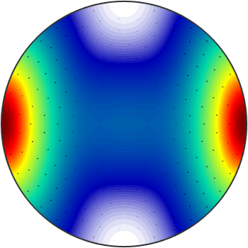
vertices: 18338 x 1As output we obtain three spherical functions vp, vs1 and vs2 representing the velocities of P, and fast and slow S-waves respectively in dependency of the propagation direction. The remaining three output variables pp, ps1, ps2 are spherical vector fields representing the polarization directions of these wave as functions of the propagation direction.
In order to visualize these quantities, there are several possibilities. Let us first plot the direction dependent wave speed of the p-wave
plot(vp,'complete','upper')
Next, we plot on the top of this plot the p-wave polarization direction.
hold on
plot(pp)
hold off
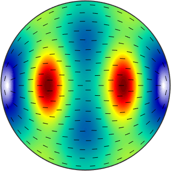
We may even compute with these spherical functions as width ordinary values. E.g. to visualize the speed difference between the s1 and s2 waves we do.
plot(vs1-vs2,'complete','upper')

hold on
plot(ps1)
hold off
When projected to a plane the different wave speeds
planeNormal = vector3d.X;

% options for sections
optSec = {'color','interp','linewidth',6,'doNotDraw'};

% options for quiver
optQuiver = {'linewidth',2,'autoScaleFactor',0.35,'doNotDraw'};
optQuiverProp = {'color','k','linewidth',2,'autoScaleFactor',0.25,'doNotDraw'};
prop = S2VectorFieldHarmonic.normal; % the propagation direction

% wave velocities
%close all
plotSection(vp,planeNormal,optSec{:},'DisplayName','Vp')
hold on
plotSection(vs1,planeNormal,optSec{:},'DisplayName','Vs1')
plotSection(vs2,planeNormal,optSec{:},'DisplayName','Vs2')

% polarization directions
quiverSection(vp,pp,planeNormal,'color','c',optQuiver{:},'DisplayName','pp')
quiverSection(vs1,ps1,planeNormal,'color','g',optQuiver{:},'DisplayName','ps1')
quiverSection(vs2,ps2,planeNormal,'color','m',optQuiver{:},'DisplayName','ps2')

% plot propagation directions as reference
quiverSection(vp,prop,planeNormal,optQuiverProp{:},'DisplayName','x')
quiverSection(vs1,prop,planeNormal,optQuiverProp{:})
quiverSection(vs2,prop,planeNormal,optQuiverProp{:})
hold off

axis off tight
legend('Vp','Vs1','Vs2','pp','ps1','ps2','x','Location','eastOutSide')
mtexTitle('Phase velocity surface (km/s)')

mtexColorMap blue2red
mtexColorbar('Title','(km/s)','location','southOutSide')
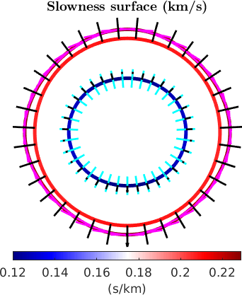
Similarly, we can visualize the slowness surfaces (s/km)
% plot slowness surfaces
plotSection(1./vp,planeNormal,optSec{:},'DisplayName','Vp')
hold on
plotSection(1./vs1,planeNormal,optSec{:},'DisplayName','Vs1')
plotSection(1./vs2,planeNormal,optSec{:},'DisplayName','Vs2')

% polarization directions
quiverSection(1./vp,pp,planeNormal,'color','c',optQuiver{:},'DisplayName','pp')
quiverSection(1./vs1,ps1,planeNormal,'color','g',optQuiver{:},'DisplayName','ps1')
quiverSection(1./vs2,ps2,planeNormal,'color','m',optQuiver{:},'DisplayName','ps2')

% plot propagation directions as reference
quiverSection(1./vp,prop,planeNormal,optQuiverProp{:},'DisplayName','x')
quiverSection(1./vs1,prop,planeNormal,optQuiverProp{:})
quiverSection(1./vs2,prop,planeNormal,optQuiverProp{:})
hold off
axis off tight
legend('Vp','Vs1','Vs2','pp','ps1','ps2','x','Location','eastOutSide')
mtexTitle('Slowness surface (km/s)')

mtexColorMap blue2red
mtexColorbar('Title','(s/km)','location','southOutSide')
set back default colormap
setMTEXpref('defaultColorMap',WhiteJetColorMap)