Interpolating EBSD Data

Interpolating EBSD Data edit page

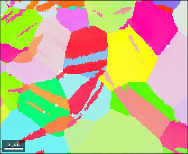
In the section Denoising and Filling Missing Data we have discussed how to work with noisy EBSD data the contained non indexed pixels. Hereby, we made the assumption that the grid before and after the operations is the same.

In this section we explain how to interpolate an EBSD map at positions that do not belong to the grid. Lets us consider a simple example

mtexdata twins;

[grains, ebsd.grainId] = calcGrains(ebsd('indexed'));

% this command here is important :)
ebsd = ebsd.project2FundamentalRegion(grains);

plot(ebsd('indexed'),ebsd('indexed').orientations)

ebsd = EBSD
 
 Phase  Orientations     Mineral         Color  Symmetry  Crystal reference frame
     0     46 (0.2%)  notIndexed                                                 
     1  22833 (100%)   Magnesium  LightSkyBlue     6/mmm       X||a*, Y||b, Z||c*
 
 Properties: bands, bc, bs, error, mad
 Scan unit : um
 X x Y x Z : [0 50] x [0 41] x [0 0]
 Normal vector: (0,0,1)

In most cases it is useful to gridify the data before doing interpolation.

ebsd = ebsd.gridify

ebsd = EBSDsquare
 
 Phase  Orientations     Mineral         Color  Symmetry  Crystal reference frame
     0     46 (0.2%)  notIndexed                                                 
     1  22833 (100%)   Magnesium  LightSkyBlue     6/mmm       X||a*, Y||b, Z||c*
 
 Properties: bands, bc, bs, error, mad, grainId, oldId
 Scan unit : um
 X x Y x Z : [0 50] x [0 41] x [0 0]
 Normal vector: (0,0,1)
 Square grid  :137 x 167

Now we can use the command interp to interpolate the orientation at arbitrary coordinates x and y.

x = 30.5; y = 5.5;
e1 = interp(ebsd,x,y)

e1 = EBSD
 
 Phase  Orientations    Mineral         Color  Symmetry  Crystal reference frame
     1      1 (100%)  Magnesium  LightSkyBlue     6/mmm       X||a*, Y||b, Z||c*
 
 Id   Phase              orientation   bands    bc    bs   error   mad   grainId   oldId
  1       1   (162.9°,111.9°,186.1°)      10   160   255       0   0.4        36    3109
 Scan unit : um
 X x Y x Z : [30 30] x [5.5 5.5] x [0 0]
 Normal vector: (0,0,1)

By default the command interp performs inverse distance interpolation. This is different to

e2 = ebsd('xy',x,y)

e2 = EBSD
 
 Phase  Orientations    Mineral         Color  Symmetry  Crystal reference frame
     1      1 (100%)  Magnesium  LightSkyBlue     6/mmm       X||a*, Y||b, Z||c*
 
    Id   Phase            orientation   bands    bc    bs   error   mad   grainId   oldId
 13994       1   (163°,111.9°,186.1°)      10   156   216       0   0.4        36    3276
 Scan unit : um
 X x Y x Z : [31 31] x [5.7 5.7] x [0 0]
 Normal vector: (0,0,1)

which returns the nearest neighbour EBSD measurement. Lets have a look at the difference

angle(e1.orientations,e2.orientations)./degree

ans =
    0.1027

Change of the measurement grid

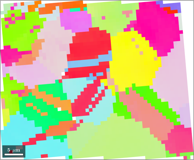
The command interp can be used to evaluate the EBSD map on a different grid, which might have higher or lower resolution or might even be rotated. Lets demonstrate this

% define a rotated coarse grid
omega = 5*degree;
[xmin, xmax, ymin, ymax] = ebsd.extent;
x = linspace(xmin-cos(omega)*ymax,xmax,100);
y = linspace(ymin-sin(omega)*xmax,ymax,50);
[x,y] = meshgrid(x,y);

xy = [cos(omega) -sin(omega); sin(omega) cos(omega) ] * [x(:),y(:)].';

% define the EBSD data set on this new grid
ebsdNewGrid = interp(ebsd,xy(1,:),xy(2,:))

% plot the regridded EBSD data set
plot(ebsdNewGrid('indexed'),ebsdNewGrid('indexed').orientations)

ebsdNewGrid = EBSD
 
 Phase  Orientations     Mineral         Color  Symmetry  Crystal reference frame
     0    2624 (52%)  notIndexed                                                 
     1    2376 (48%)   Magnesium  LightSkyBlue     6/mmm       X||a*, Y||b, Z||c*
 
 Properties: bands, bc, bs, error, mad, grainId, oldId
 Scan unit : um
 X x Y x Z : [-44 50] x [-7.9 45] x [0 0]
 Normal vector: (0,0,1)

Note, that we have not rotated the EBSD data but only the grid. All orientations as well as the position of all grains remains unchanged.

Another example is the change from a square to an hexagonal grid or vice versa. In this case the command interp is implicitely called by the command gridify. In order to demonstrate this functionality we start by EBSD data on a hex grid

mtexdata ferrite silent

plot(ebsd,ebsd.orientations)

and resample the data on a square grid. To do so we first define a smaller square unit cell corresponding to the hexagonal unit cell

% define a square unit cell
squnitCell = ebsd.dPos / 4 * vector3d([1 1 -1 -1],[1 -1 -1 1],0).';

% use the square unit cell for gridify
ebsd = ebsd.gridify('unitCell',squnitCell);

plot(ebsd,ebsd.orientations)