The kernel average misorientation (KAM) is a measure of local grain misorientation that is usually derived from EBSD data. For a formal definition of the KAM we denote by \(o_{i,j}\) the orientations at pixel position \((i,j)\) and by \(N(i,j)\) the set of all neighboring pixels. Then the kernel average misorientation \(\mathrm{kam}_{i,j}\) at pixel position \((i,j)\) is defined as
\[\mathrm{KAM}_{i,j} = \frac{1}{|N(i,j)|}\sum_{(k,l) \in N(i,j)} \omega(o_{i,j}, o_{k,l}) \]
Here \(\lvert N(i,j)\rvert\) denotes the number of all neighboring pixels taking into account and \(\omega(o_{i,j}, o_{k,l})\) the disorientation angle between the orientation \(o_{ij}\) in the center and the neighboring orientation \((o_{k,l})\). The specific choice of the set \(N(i,j)\) of neighboring pixels is crucial for the computation of the KAM. Most commonly the following additional constrains are made
- consider neighbors up to order \(n\), e.g. \(n=1,2,3,\ldots\)
- consider only neighbors belonging to the same grain
- consider only neighbors with a misorientation angle smaller than a threshold angle \(\delta\)
In the case of square and hexagonal grids the order of neighbors is illustrated below
plotSquareNeighbours; nextAxis(1,2); plotHexNeighbours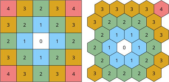
A Deformed Ferrite Specimen
Let us demonstrate the computation of the KAM at the example of a deformed Ferrite specimen. Lets import the data first and reconstruct the grain structure
mtexdata ferrite

[grains,ebsd.grainId] = calcGrains(ebsd('indexed'),'minPixel',3);
grains = smooth(grains,5);

plot(ebsd('indexed'),ebsd('indexed').orientations)
hold on
plot(grains.boundary,'lineWidth',1.5)
hold off
ebsd = EBSD (y↑→x)
Phase Orientations Mineral Color Symmetry Crystal reference frame
-1 1 (0.0016%) notIndexed
0 63044 (100%) Ferrite LightSkyBlue 432
Properties: ci, fit, iq, sem_signal
Scan unit : um
X x Y x Z : [0, 70] x [0, 70] x [0, 0]
Normal vector: (0,0,1)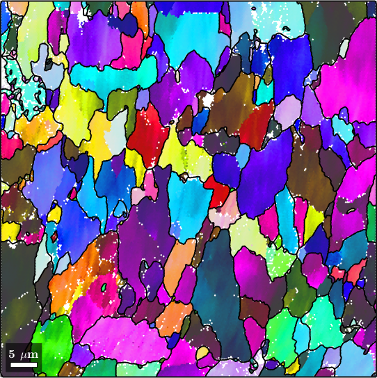
Although MTEX allows the computation of the KAM from arbitrarily sampled EBSD maps the algorithms are much faster an memory efficient if the maps are measured on regular hexagonal or rectangular grid - as it is standard in most applications. The command gridify makes MTEX aware of such an underlying regular measurement grid.
ebsd = ebsd.gridify;The kernel average misorientation is computed by the command ebsd.KAM. As all MTEX commands it return the mean disorientation angle in radiant. Hence, dividing by the constant degree gives the result in degree.
kam = ebsd.KAM / degree;

% lets plot it
plot(ebsd,kam,'micronbar','off')
setColorRange([0,15])
mtexColorbar
mtexColorMap LaboTeX
hold on
plot(grains.boundary,'lineWidth',1.5)
hold off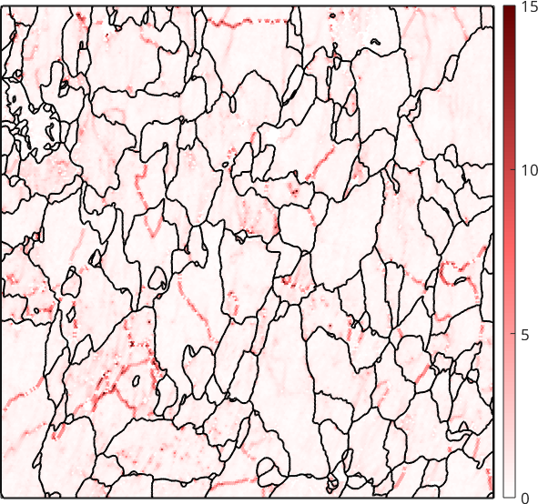
When computed with default parameters in MTEX neighbors up to order 1 are considered and no threshold angle \(\delta\) is applied. If grains have been reconstructed and the property ebsd.grainId has been set (as we did above) only misorientations within the same grain are considered. As a consequence the resulting KAM map is dominated by the orientation gradients at the sub-grain boundaries.
Specifying a reasonable small threshold angle \(\delta=2.5^{\circ}\) the sub-grain boundaries can be effectively removed from the KAM.
plot(ebsd,ebsd.KAM('threshold',2.5*degree) ./ degree,'micronbar','off')
setColorRange([0,2])
mtexColorbar
mtexColorMap LaboTeX
hold on
plot(grains.boundary,'lineWidth',1.5)
hold off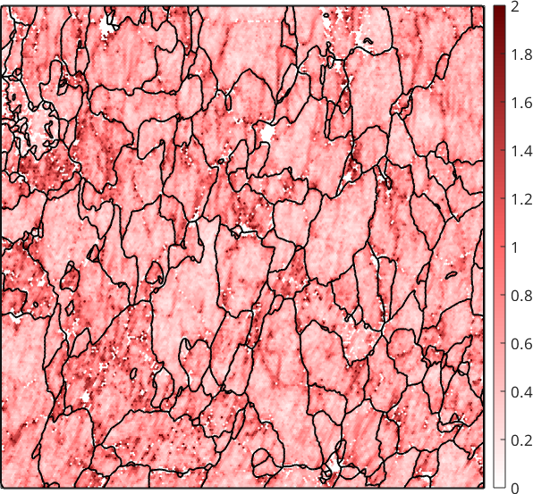
Unfortunately, the remaining KAM becomes very sensitive to measurement errors and is often very noisy. The noise can be reduced by considering higher order neighbors
plot(ebsd,ebsd.KAM('threshold',2.5*degree,'order',5) ./ degree,'micronbar','off')
setColorRange([0,2])
mtexColorbar
mtexColorMap LaboTeX
hold on
plot(grains.boundary,'lineWidth',1.5)
hold off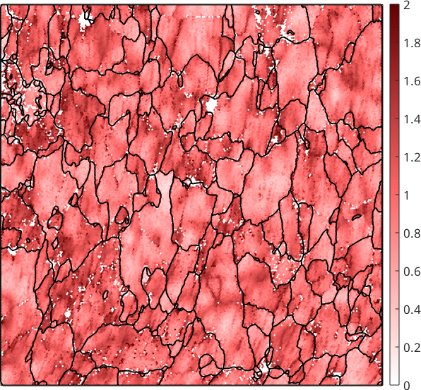
Although this reduces noise it also smooths away local dislocation structures. A much more effective way to reduce the effect of measurement errors to the kernel average misorientation is to denoise the EBSD map first and compute than the KAM from the first order neighbors.
% chose a denoising filter
F = halfQuadraticFilter;
F.alpha = 0.5;

% denoise the orientation map
ebsdS = smooth(ebsd,F,'fill',grains);

% plot the first order KAM
plot(ebsdS,ebsdS.KAM('threshold',2.5*degree) ./ degree,'micronbar','off')
setColorRange([0,2])
mtexColorbar
mtexColorMap LaboTeX
hold on
plot(grains.boundary,'lineWidth',1.5)
hold off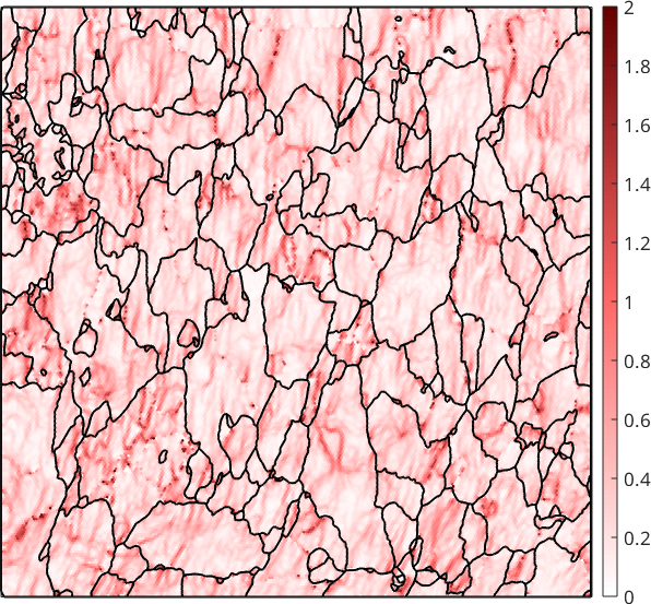
We observe that the KAM is not longer related to sub-grain boundaries and nicely reveals local dislocation structures of the deformed material.
Some helper functions
The functions below where only used to generate the neighborhood pictures of the first paragraph
function plotSquareNeighbours

N = [4 3 2 3 4;...
  3 2 1 2 3;...
  2 1 0 1 2;...
  3 2 1 2 3;...
  4 3 2 3 4];

cs = crystalSymmetry;
ebsd = EBSDsquare([],rotation.nan(5,5),N,0:4,{cs,cs,cs,cs,cs},'dxy',[10 10]);
plot(ebsd,'EdgeColor','black','micronbar','off','figSize','small')
legend off

text(ebsd,N)

end

function plotHexNeighbours

N = [3 2 2 2 3;...
  2 1 1 2 3;...
  2 1 0 1 2;...
  2 1 1 2 3;...
  3 2 2 2 3;...
  3 3 3 3 4];

cs = crystalSymmetry;
ebsd = EBSDhex([],rotation.nan(6,5),N,0:4,{cs,cs,cs,cs,cs},10,1,1);
plot(ebsd,'edgecolor','k','micronbar','off','figSize','small')
legend off
text(ebsd,N)
axis off

end