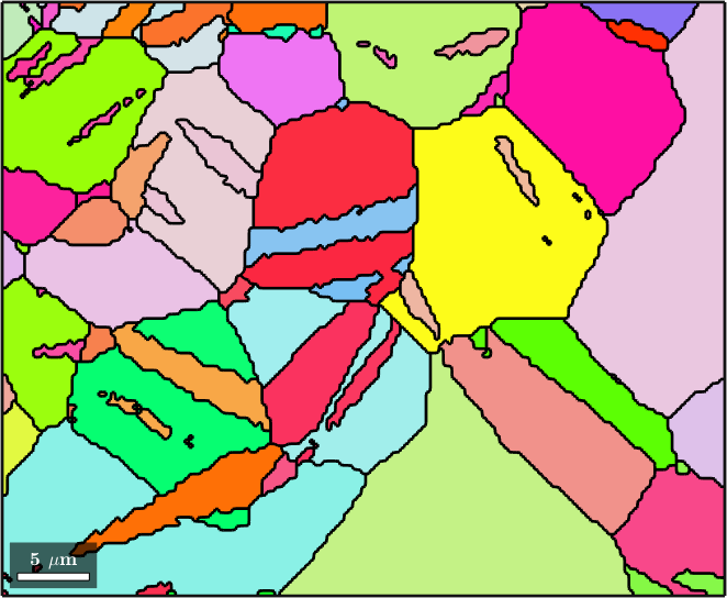
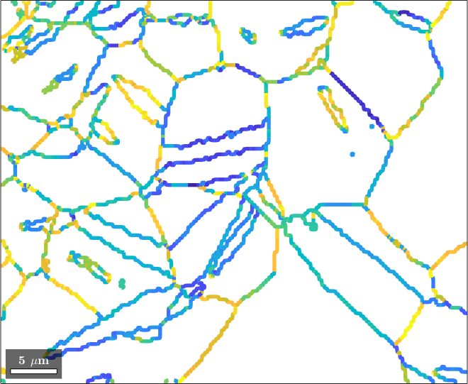
In this section we discus geometric properties that can be derived from grain boundaries. Lets start by importing some EBSD data and computing grain boundaries.
% load some example data
mtexdata twins silent
ebsd.prop = rmfield(ebsd.prop,{'error','bands'});

% detect grains
[grains,ebsd.grainId,ebsd.mis2mean] = ...
  calcGrains(ebsd('indexed'),'angle',10*degree,'minPixel',3);

% smooth them
grains = grains.smooth(5);

% visualize the grains
plot(grains,grains.meanOrientation)

% extract all grain boundaries
gB = grains.boundary;

hold on
plot(gB,'LineWidth',2)
hold off
Property overview
A variable of type grainBoundary contains the following properties
|
ebsdId |
neighboring pixel ids |
phaseId |
neighboring phase ids |
|
grainId |
neighboring grain ids |
F |
vertices ids of the segments |
|
length of each segment |
direction |
direction of each segment |
|
|
midPoint |
mid point of the segment |
curvature of each segment |
|
|
misorientation |
between ebsdId(:,1) and ebsdId(:,2) |
triplePoints |
list of all triple points |
|
componentId |
connected component id |
componentSize |
connected component size |
The first three properties refer to \(N \times 2\) matrices where \(N\) is the number of boundary segments. Each row of these matrices contains the information about the EBSD data, and grain data on both sides of the grain boundary. To illustrate this consider the grain boundary of one specific grain
gB4 = grains(4).boundarygB4 = grainBoundary
Segments length mineral 1 mineral 2
8 1.3 µm Magnesium MagnesiumThis boundary consists of 8 segments and hence ebsdId forms a 8x2 matrix
gB4.ebsdIdans =
1010 1177
1010 1009
843 842
843 676
843 844
1011 844
1011 1012
1011 1178It is important to understand that the id is not necessarily the same as the index in the list. In order to index an variable of type EBSD by id and not by index the following syntax has to be used
ebsd('id',gB4.ebsdId)ans = EBSD (y↑→x)
Phase Orientations Mineral Color Symmetry Crystal reference frame
1 16 (100%) Magnesium LightSkyBlue 6/mmm X||a*, Y||b, Z||c*
Id Phase orientation bc bs mad grainId mis2mean
1010 1 (113.7°,15.5°,219.3°) 164 158 0.5 4 (217.3°,0.2°,142.9°)
1010 1 (113.7°,15.5°,219.3°) 164 158 0.5 4 (217.3°,0.2°,142.9°)
843 1 (115.3°,15.6°,218.2°) 170 176 0.7 4 (55.9°,0.2°,303.8°)
843 1 (115.3°,15.6°,218.2°) 170 176 0.7 4 (55.9°,0.2°,303.8°)
843 1 (115.3°,15.6°,218.2°) 170 176 0.7 4 (55.9°,0.2°,303.8°)
1011 1 (114.7°,15.7°,218.5°) 182 174 0.5 4 (339.9°,0.1°,20.2°)
1011 1 (114.7°,15.7°,218.5°) 182 174 0.5 4 (339.9°,0.1°,20.2°)
1011 1 (114.7°,15.7°,218.5°) 182 174 0.5 4 (339.9°,0.1°,20.2°)
1177 1 (4.5°,80.7°,195.2°) 168 171 0.3 15 (4.8°,0.3°,355.2°)
1009 1 (4.6°,80.7°,195.4°) 156 160 0.4 15 (24.6°,0.3°,335.2°)
842 1 (4.9°,80.4°,195.2°) 167 170 0.5 15 (83°,0.5°,277°)
676 1 (4.9°,80.4°,195.2°) 176 196 0.5 15 (83°,0.5°,277°)
844 1 (4.4°,80.5°,195.1°) 174 197 0.3 15 (359.6°,0.1°,0.5°)
844 1 (4.4°,80.5°,195.1°) 174 197 0.3 15 (359.6°,0.1°,0.5°)
1012 1 (4.4°,80.5°,195.2°) 176 168 0.4 15 (14.3°,0.1°,345.8°)
1178 1 (4.7°,80.8°,195.4°) 174 181 0.5 15 (21.9°,0.4°,338°)
Scan unit : um
X x Y x Z : [1.8, 2.7] x [1.2, 2.1] x [0, 0]
Normal vector: (0,0,1)
Square grid :8 x 2Similarly
gB4.grainIdans =
4 15
4 15
4 15
4 15
4 15
4 15
4 15
4 15results in 8x2 matrix indicating that grain 4 is a tiny inclusion of grain 15.
plot(grains(4),'FaceColor','DarkBlue','micronbar','off')
hold on
plot(grains(15),'FaceColor','LightCoral')
hold off
Grain boundary misorientations
The grain boundary misorientation defined as the misorientation between the orientations corresponding to ids in first and second column of ebsdId, i.e. following two commands should give the same result
gB4(1).misorientation

inv(ebsd('id',gB4.ebsdId(1,2)).orientations) .* ebsd('id',gB4.ebsdId(1,1)).orientations
ans = misorientation (Magnesium → Magnesium)
antipodal: true
Bunge Euler angles in degree
phi1 Phi phi2
330.069 86.0994 150.22
ans = misorientation (Magnesium → Magnesium)
Bunge Euler angles in degree
phi1 Phi phi2
330.069 86.0994 150.22Note that in the first result the antipodal flag is true while it is false in the second result.
Obviously, misorientations of a list of grain boundaries can only be extracted if all of them have the same type of phase transition. Let us consider only Magnesium to Magnesium grain boundaries, i.e., ommit all grain boundaries to an not indexed region.
gB_Mg = gB('Magnesium','Magnesium')gB_Mg = grainBoundary
Segments length mineral 1 mineral 2
3163 724 µm Magnesium MagnesiumThen the misorientation angles can be plotted by
plot(gB_Mg,gB_Mg.misorientation.angle./degree,'linewidth',4)
mtexColorbar('title','misorientation angle (°)')
Geometric properties
The direction property of the boundary segments is useful when checking for tilt and twist boundaries, i.e., when we want to compare the misorientation axis with the interface between the grains
% compute misorientation axes in specimen coordinates
ori = ebsd('id',gB_Mg.ebsdId).orientations;
axes = axis(ori(:,1),ori(:,2),'antipodal')

% plot the angle between the misorientation axis and the boundary direction
plot(gB_Mg,angle(gB_Mg.direction,axes),'linewidth',4)
axes = vector3d (y↑→x)
size: 3163 x 1
antipodal: true
We observe that the angle is quite oscillatory. This is because of the stair casing effect when reconstructing grains from gridded EBSD data. The weaken this effect we may average the segment directions using the command calcMeanDirection
% plot the angle between the misorientation axis and the boundary direction
plot(gB_Mg,angle(gB_Mg.calcMeanDirection(4),axes),'linewidth',4)
The midPoint property is useful when TODO:
While the command length(gB_Mg) gives the total number of all Magnesium to Magnesium grain boundary segments the command segLength(gB_Mg) gives the length of each segment in µm. The total length of all Magnesium to Magnesium grain boundary segments is hence
sum(gB_Mg.segLength)ans =
723.9185Connected components
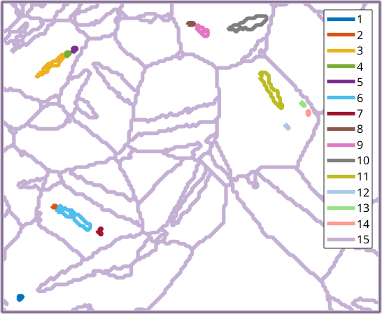
When analyzing the topology of boundary networks connected components of certain subsets of boundaries are of interest. Using the commands|gB.componentId| and gB.componentSize we are able to separate the boundary network into groups of connected components and analyze them separately. We do so below at the example of twin boundaries which we first colorize according to length.
CS = ebsd.CS;
twinning = orientation.map(Miller(1,-1,0,1,CS),Miller(1,0,-1,-1,CS),...
  Miller(0,1,-1,1,CS,'uvw'),Miller(1,-1,0,1,CS,'uvw'))

gBTwin = gB(gB.isTwinning(twinning));

plot(grains,grains.meanOrientation,'faceAlpha',0.25)

hold on
plot(gBTwin,gBTwin.componentSize,'lineWidth',4)
hold off
mtexColorbar
twinning = misorientation (Magnesium → Magnesium)
(10-1-1) || (01-11) [01-11] || [1-101]
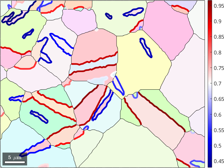
Next we compute how curvy each twin boundary component is, by dividing it spatial extension by its total length. This measure has proven to be useful to tell apart misindexing due to pseudosymmetries and true twin boundaries.
numComponents = max(gBTwin.componentId);
xmax = accumarray(gBTwin.componentId,gBTwin.midPoint.x,[numComponents,1],@max);
ymax = accumarray(gBTwin.componentId,gBTwin.midPoint.y,[numComponents,1],@max);
xmin = accumarray(gBTwin.componentId,gBTwin.midPoint.x,[numComponents,1],@min);
ymin = accumarray(gBTwin.componentId,gBTwin.midPoint.y,[numComponents,1],@min);

ext = sqrt((xmax-xmin).^2+(ymax-ymin).^2);
len = accumarray(gBTwin.componentId,gBTwin.segLength,[numComponents,1],@sum);
value = ext ./ len;

plot(grains,grains.meanOrientation,'faceAlpha',0.25)
hold on
plot(gBTwin,value(gBTwin.componentId),'lineWidth',4)
hold off
mtexColorbar
mtexColorMap blue2red