Multivariate Orientation Dependent Functions

Structural conventions of the input and output of multivariate SO3FunHarmonics

In this part we deal with multivariate functions of the form

\[ f\colon \mathcal{SO}(3) \to \mathbb R^n. \]

For example we got four nodes \(R_1, R_2, R_3\) and \(R_4\) and six functions \(f_1, f_2, f_3, f_4, f_5\) and \(f_6\), which we want to store in a 3x2 array, then the following scheme applies to function evaluations:

\[ F(:, :, 1) = \pmatrix{f_1(v_1) & f_2(v_1) & f_3(v_1) \cr f_1(v_2) & f_2(v_2) & f_3(v_2) \cr f_1(v_3) & f_2(v_3) & f_3(v_3) \cr f_1(v_4) & f_2(v_4) & f_3(v_4)} \quad\mathrm{and}\quad F(:, :, 2) = \pmatrix{f_4(v_1) & f_5(v_1) & f_6(v_1) \cr f_4(v_2) & f_5(v_2) & f_6(v_2) \cr f_4(v_3) & f_5(v_3) & f_6(v_3) \cr f_4(v_4) & f_5(v_4) & f_6(v_4)}. \]

For the intern Fourier-coefficient matrix the first dimension is reserved for the Fourier-coefficients of a single function; the dimensions of the functions itself begins again with the second dimension.

If \(\bf{\hat f}_1, \bf{\hat f}_2, \bf{\hat f}_3, \bf{\hat f}_4, \bf{\hat f}_5\) and \(\bf{\hat f}_6\) would be the column vectors of the Fourier-coefficients of the functions above, internally they would be stored in \(\hat F\) as follows. \[ \hat F(:, :, 1) = \pmatrix{\bf{\hat f}_1 & \bf{\hat f}_2 & \bf{\hat f}_3} \quad\mathrm{and}\quad \hat F(:, :, 2) = \pmatrix{\bf{\hat f}_4 & \bf{\hat f}_5 & \bf{\hat f}_6}. \]

Defining a multivariate SO3FunHarmonic

Definition via function values

At first we need some vertices

nodes = equispacedSO3Grid(crystalSymmetry,specimenSymmetry,'points',1e5);
nodes = nodes(:);

Next we define function values for the vertices

y = [SO3Fun.dubna(nodes), (nodes.a .* nodes.b).^(1/4)];
nodes.CS = SO3Fun.dubna.CS;

Now the actual command to get a (2x1) SO3F1 of type \(~\) SO3FunHarmonic is

SO3F1 = SO3FunHarmonic.approximation(nodes, y,'maxit',10)

Warning: The Voronoi decomposition is calculated. This may take some
time. 
 
SO3F1 = SO3FunHarmonic (Quartz → xyz)
  isReal: false
  size: 2 x 1
  bandwidth: 54
  weight: 1

It is also possible to interpolate one component by an SO3FunRBF, that means

SO3F2 = SO3FunHarmonic.interpolate(nodes,y(:,1))

SO3F2 = SO3FunRBF (Quartz → xyz)
 
  uniform component
  weight: 0.00065
 
  multimodal components
  kernel: de la Vallee Poussin, halfwidth 5°
  center: 17292 orientations, resolution: 5°
  weight: 1

This is only possible for univariate functions.

Definition via function handle

If we have a function handle for the function we could create a SO3FunHarmonic via quadrature. At first let us define a function handle which takes \(~\) rotation as an argument and returns double:

f = @(rot) [exp(rot.a+rot.b+rot.c)+50*(rot.b-cos(pi/3)).^3.*(rot.b-cos(pi/3) > 0), rot.a, rot.b, rot.c];

Now we call the quadrature command to get (4x1) SO3F3 of type \(~\) SO3FunHarmonic

SO3F3 = SO3FunHarmonic.quadrature(f, 'bandwidth', 50,SO3F1.CS)

SO3F3 = SO3FunHarmonic (Quartz → xyz)
  isReal: false
  size: 4 x 1
  bandwidth: 50
  weight: 1.1

Definition via Fourier-coefficients

If we already know the Fourier-coefficients, we can simply hand them in the format above to the constructor of SO3FunHarmonic.

SO3F4 = SO3FunHarmonic(eye(10))

SO3F4 = SO3FunHarmonic (xyz → xyz)
  isReal: false
  size: 10 x 1
  bandwidth: 1
  weight: 1

Operations which differ from an univariate SO3FunHarmonic

Some default matrix and vector operations

You can concatenate and refer to functions as MATLAB does with vectors and matrices

SO3F5 = [SO3F1; SO3F3];
SO3F5(2:4)

ans = SO3FunHarmonic (Quartz → xyz)
  isReal: false
  size: 3 x 1
  bandwidth: 54
  weight: 0.49+0.2i

You can conjugate the Fourier-coefficients and transpose/ctranspose the multivariate SO3FunHarmonic.

conj(SO3F1);
SO3F1.';
SO3F1'

ans = SO3FunHarmonic (Quartz → xyz)
  isReal: false
  size: 1 x 2
  bandwidth: 54
  weight: 1

Some other operations

length(SO3F1)
size(SO3F3)
SO3F4 = reshape(SO3F4, 2, [])

ans =
     2
ans =
     4     1
 
SO3F4 = SO3FunHarmonic (xyz → xyz)
  isReal: false
  size: 2 x 5
  bandwidth: 1
  weight: 1

sum and mean

If we do not specify further options to sum or mean they give we the integral or the mean value back for each function. You could also calculate the conventional sum or the meanvalue over a dimension of a multivariate SO3FunHarmonic.

sum(SO3F1, 1)
mean(SO3F4, 2)

ans = SO3FunHarmonic (Quartz → xyz)
  isReal: false
  bandwidth: 54
  weight: 1.49+0.2i
 
 
ans = SO3FunHarmonic (xyz → xyz)
  antipodal: true
  size: 2 x 1
  bandwidth: 1
  weight: 0.2

min/max

If the min or max command gets a multivariate SO3FunHarmonic the pointwise minimum or maximum is calculated along the first non-singelton dimension if not specified otherwise.

Therefore the function has to be real valued

SO3F4.isReal = 1;
min(SO3F4)

ans =
  Columns 1 through 7
    1.0000   -1.7320   -1.2247   -1.7320   -1.2247   -1.7321   -1.2247
  Columns 8 through 10
   -1.7320   -1.2247   -1.7320

Remark on the matrix product

At this point the matrix product is implemented pointwise and not as the usual matrix product.

SO3F1.CS=specimenSymmetry;

SO3F1 .* SO3F4

ans = SO3FunHarmonic (xyz → xyz)
  isReal: false
  size: 2 x 5
  bandwidth: 55
  weight: 1

Visualization of multivariate SO3FunHarmonic

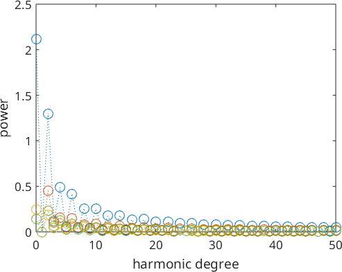
Similarly to the univariate case we also can look at the Fourier coefficients of multivariate functions.

plotSpektra(SO3F3)

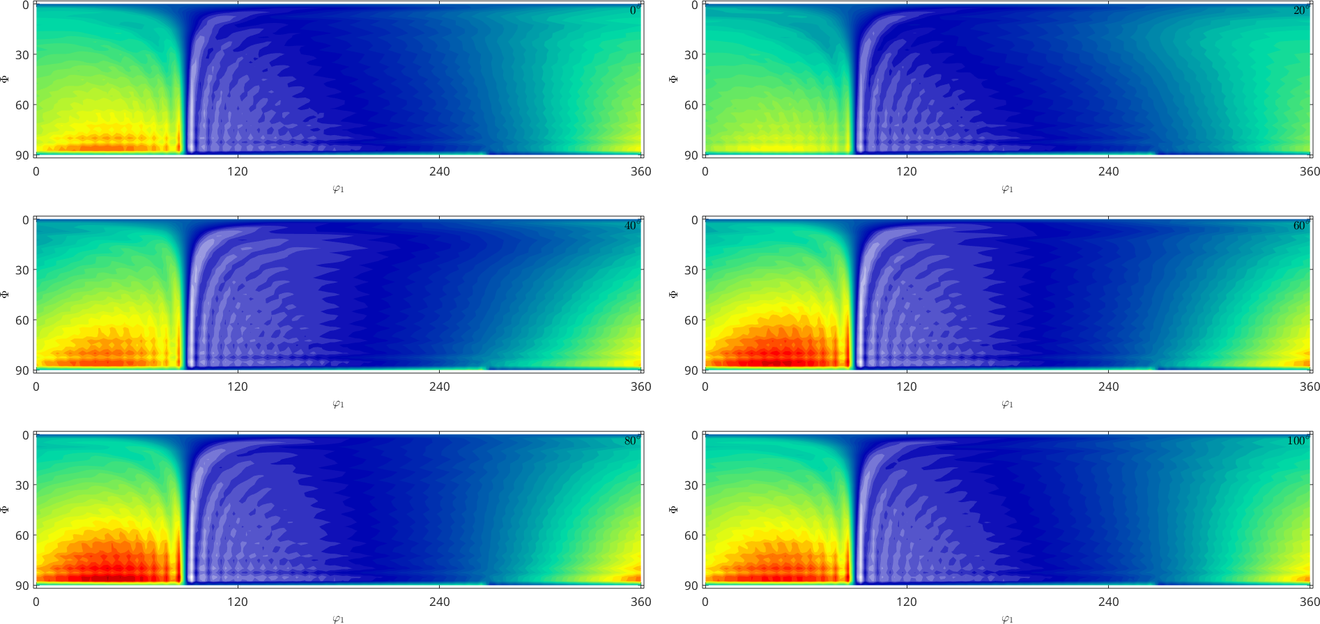
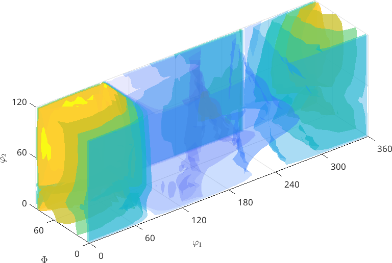
The section plot and the 3d plot are performed only for the first component of a multivariate function

plot(SO3F3)

Warning: You try to plot an multivariate function. Plot the desired
components manually. In the following the first component is plotted. 
Warning: Imaginary part of complex valued SO3FunHarmonic is ignored.
In the following only the real part is plotted.

plot3d(SO3F3)

Warning: You try to plot an multivariate function. Plot the desired
components manually. In the following the first component is plotted. 
Warning: Imaginary part of complex valued SO3FunHarmonic is ignored.
In the following only the real part is plotted.

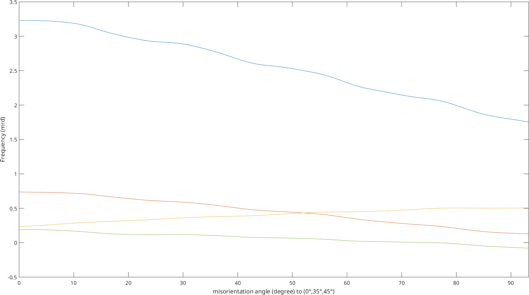
while the plot along a specific fibre includes all components.

plotFibre(SO3F3,fibre.beta)

Warning: Imaginary part of complex valued SO3FunHarmonic is ignored.
In the following only the real part is plotted.