Explains how to combine several plots, e.g. plotting on the top of an inverse pole figure some important crystal directions.
General Principle
In order to tell MATLAB to plot one plot right on the top of an older plot one has to use the commands hold all and hold off. Let's demonstrate this using a simple example.
plot([2 2],'LineWidth',2)

hold on

plot([1 3],'LineWidth',2)

hold off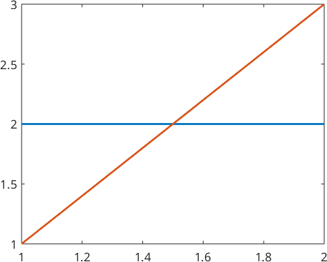
Combine Different EBSD Data
First, we want to show up two different orientation data sets in one plot
% let's simulate some orientation data
cs = crystalSymmetry('-3m');
odf = unimodalODF(orientation.byEuler(0,0,0,cs));
ori = discreteSample(odf,100);
ori_rotated = discreteSample(rotate(odf,rotation.byEuler(60*degree,60*degree,0*degree)),100);
plot them as a scatter plot in axis/angle space
scatter(ori,'axisAngle')
hold on % keep plot
scatter(ori_rotated);
hold off % next plot command deletes all plots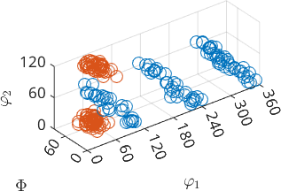
a second way would be to superpose the pole figures of both sets of orientations.
h = [Miller(0,0,0,1,cs),Miller(1,0,-1,0,cs)];
plotPDF(ori,h,'antipodal','MarkerSize',4)
hold on
plotPDF(ori_rotated,h,'MarkerSize',4);
hold off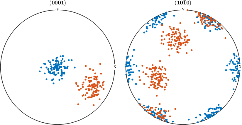
Overlaying contour and scatter plots
A more robust way to overlay multiple plots is to use the options 'add2all' instead of 'hold on'. This works for pole figure plots
plotPDF(odf,h,'antipodal','contourf','grid')
mtexColorMap white2black

plot(ori,'DisplayName','EBSD 1',...
  'MarkerSize',5,'MarkerColor','b','MarkerEdgeColor','w','add2all')

plot(ori_rotated,'DisplayName','EBSD 2',...
  'MarkerSize',5,'MarkerColor','r','MarkerEdgeColor','k','add2all');

legend('show','location','northeast')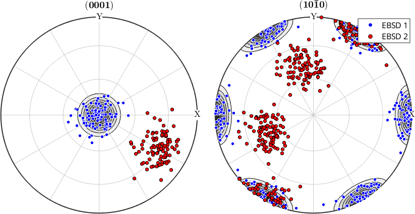
as well as with ODF section
plot(odf,'sections',8,'contourf','sigma')
mtexColorMap white2black
plot(ori,'MarkerSize',6,'MarkerColor','b','MarkerEdgeColor','w','add2all')
plot(ori_rotated,'MarkerSize',6,'MarkerColor','r','MarkerEdgeColor','k','add2all');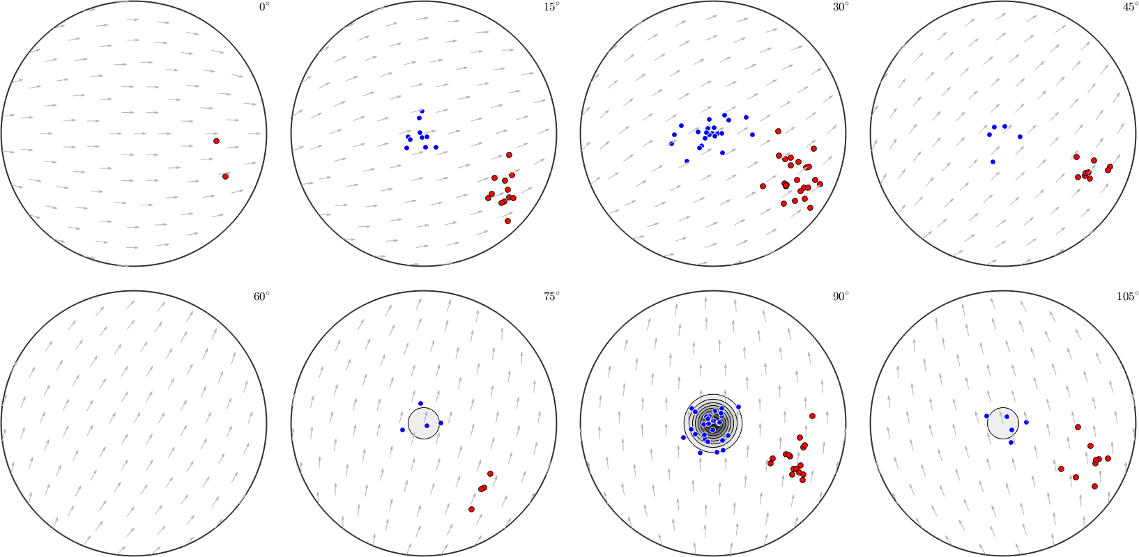
Add Miller Indices to an Inverse Pole Figure Plot
Next, we are going to add some Miller indices to an inverse pole figure plot.
plotIPDF(odf,xvector,'noLabel');
mtexColorMap white2black

hold on % keep plot
plot(Miller(0,0,0,1,cs),'symmetrised','labeled','backgroundColor','w')
plot(Miller(1,1,-2,0,cs),'symmetrised','labeled','backgroundColor','w')
plot(Miller(0,1,-1,0,cs),'symmetrised','labeled','backgroundColor','w')
plot(Miller(0,1,-1,1,cs),'symmetrised','labeled','backgroundColor','w')
hold off % next plot command deletes all plots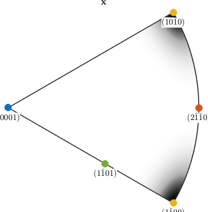
Combining different plots in one figure
The next example demonstrates how to arrange arbitrary plots into one figure
% let us import some pole figure data
mtexdata dubna
pf = PoleFigure (y↑→x)
crystal symmetry : Quartz (321, X||a*, Y||b, Z||c*)
h = (02-21), r = 72 x 19 points
h = (10-10), r = 72 x 19 points
h = (10-11)(01-11), r = 72 x 19 points
h = (10-12), r = 72 x 19 points
h = (11-20), r = 72 x 19 points
h = (11-21), r = 72 x 19 points
h = (11-22), r = 72 x 19 pointsnext, we compute an ODF out of them
odf = calcODF(pf)odf = SO3FunRBF (Quartz → y↑→x)
multimodal components
kernel: de la Vallee Poussin, halfwidth 5°
center: 19848 orientations, resolution: 5°
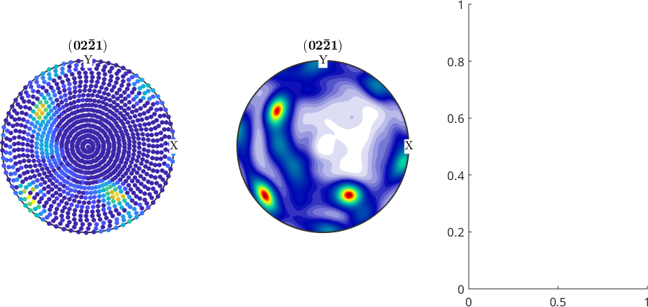
weight: 1now we want to plot the original data alongside with the recalculated pole figures and with a difference plot
figure('position',[50 50 1200 500])

% set position 1 in a 1x3 matrix as the current plotting position
axesPos = subplot(1,3,1);

% plot pole figure 1 at this position
plot(pf({1}),'parent',axesPos)

% set position 2 in a 1x3 matrix as the current plotting position
axesPos = subplot(1,3,2);

% plot the recalculated pole figure at this position
plotPDF(odf,pf{1}.h,'antipodal','parent',axesPos)

% set position 3 in a 1x3 matrix as the current plotting position
axesPos = subplot(1,3,3);

% plot the difference pole figure at this position
%plotDiff(odf,pf({1}),'parent',axesPos)