On this page we consider the problem of determining a smooth orientation dependent function \(f(\mathtt{ori})\) given a list of orientations \(\mathtt{ori}_n\) and a list of corresponding values \(v_n\). These values may by the volume of crystals with this specific orientation, as in the case of an ODF, or to any other orientation dependent physical property.
Such data may be stored in ASCII files which have lines of Euler angles, representing the orientations, and values. Such data files may be read using the command load, where we have to specify the position of the columns of the Euler angles as well as of the additional properties.
fname = fullfile(mtexDataPath, 'orientation', 'dubna.csv');
[ori, S] = orientation.load(fname,'columnNames',{'phi1','Phi','phi2','values'});
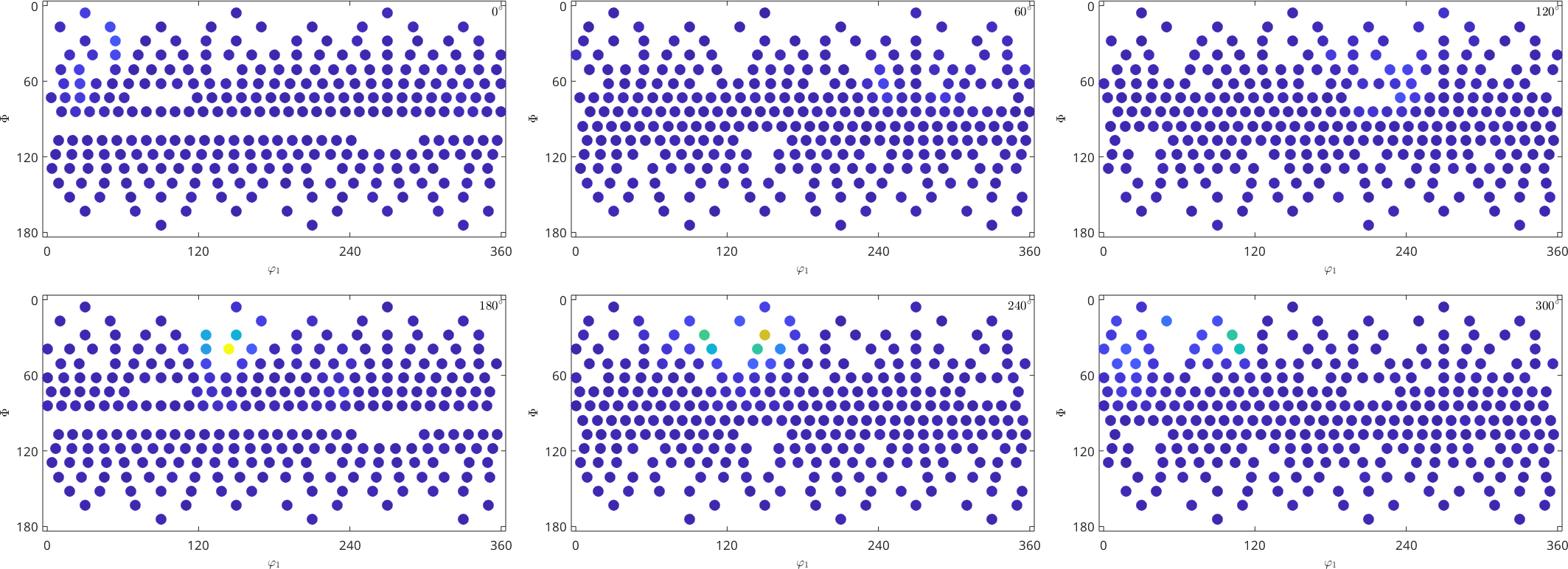
As a result the command returns a list of orientations ori and a struct S. The struct contains one field for each additional column in our data file. In out toy example it is the field S.values. Lets generate a discrete plot of the given orientations ori together with the values S.values.
plotSection(ori, S.values,'all');
Now, we want to find a function which coincides with the given function values in the nodes reasonably well.
Interpolation
Interpolation is done by the interpolate command of class SO3Fun
psi = SO3DeLaValleePoussinKernel('halfwidth',7.5*degree)
SO3F = SO3Fun.interpolate(ori, S.values,'exact','kernel',psi);
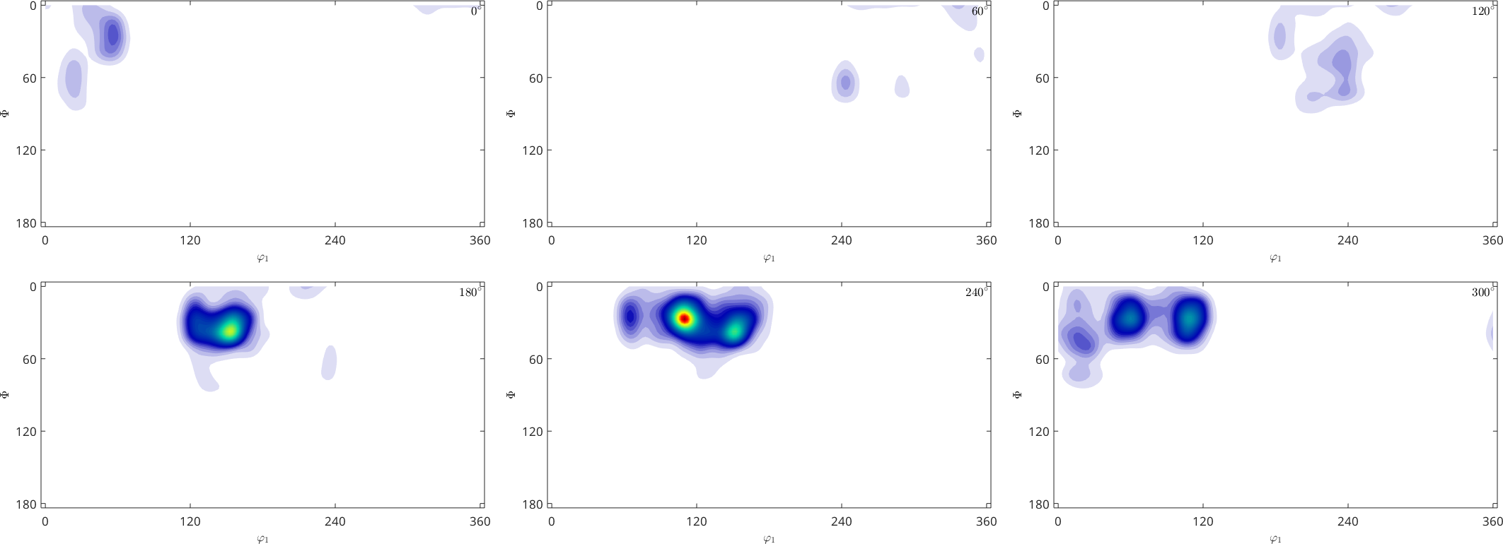
plot(SO3F)
psi = SO3DeLaValleePoussinKernel
bandwidth: 33
halfwidth: 7.5°
The interpolation is done by lsqr. Hence the error is not in machine precision.
norm(SO3F.eval(ori) - S.values) / norm(S.values)ans =
0.0943If we don't restrict ourselves to the given function values in the nodes, we have more freedom, which can be seen in the case of approximation.
Approximation of noisy data
The exact interpolation from before is also computational hard if we have a high number of nodes and function values given.
Alternatively assume that our function values are noisy.
val = S.values + randn(size(S.values)) * 0.05 * std(S.values);

plotSection(ori,val,'all')
In contrast to interpolation we are now not restricted to the exact function values in the nodes but still want to keep the error reasonably small.
One way is to interpolate the function similarly as before, without the option 'exact'.
Another way is to approximate the rotational function with a SO3FunHarmonic, which is a series of Wigner-D functions (Harmonic series). We don't take as many Wigner-D functions as there are nodes, such that we are in the overdetermined case. In that way we don't have a chance of getting the error in the nodes zero but hope for a smoother approximation. This can be achieved by the approximation command of the class SO3FunHarmonic
SO3F2 = SO3FunHarmonic.approximation(ori, val,'bandwidth',18)
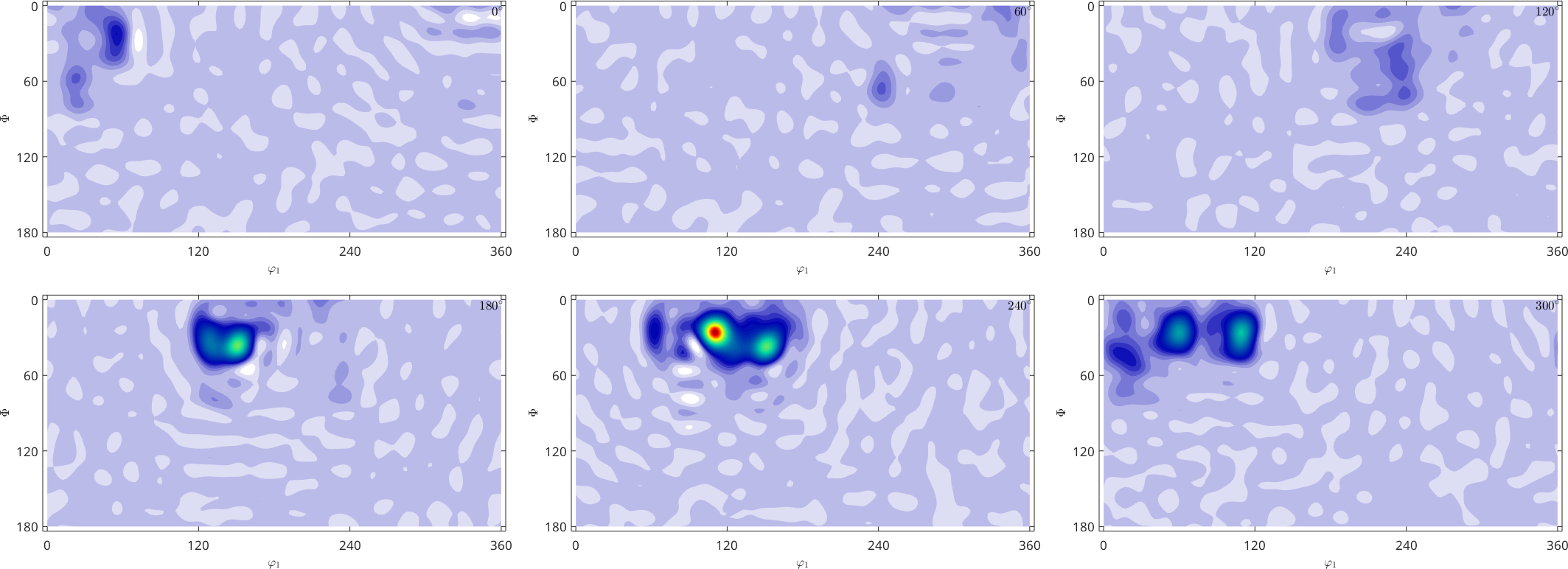
plot(SO3F2)
SO3F2 = SO3FunHarmonic (1 → xyz)
bandwidth: 18
weight: 1
Plotting this function, we can immediately see, that we have a much smoother function. But one has to keep in mind that we can not expect the error in the data nodes to be zero, as this would mean overfitting to the noisy input data.
norm(eval(SO3F2, ori) - S.values) / norm(S.values)ans =
0.0660But this may not be of great importance like in the case of function approximation from noisy function values, where we don't know the exact function values anyways.
The strategy underlying the approximation-command to obtain such an approximation works via Wigner-D functions (SO3FunHarmonicSeries Basics of rotational harmonics). For that, we seek for so-called Fourier-coefficients \({\bf \hat f} = (\hat f^{0,0}_0,\dots,\hat f^{N,N}_N)^T\) such that
\[ g(x) = \sum_{n=0}^N\sum_{k,l = -n}^n \hat f_n^{k,l} D_n^{k,l}(x) \]
approximates our function. A basic strategy to achieve this is through least squares, where we minimize the functional
\[ \sum_{m=1}^M|f(x_m)-g(x_m)|^2 \]
for the data nodes \(x_m\), \(m=1,\dots,M\). Here \(f(x_m)\) are the target function values and \(g(x_m)\) our approximation evaluated in the given data nodes.
This can be done by the lsqr method of MATLAB, which efficiently seeks for roots of the derivative of the given functional (also known as normal equation). In the process we compute the matrix-vector product with the Fourier-matrix multiple times, where the Fourier-matrix is given by
\[ F = [D_n^{k,l}(x_m)]_{m = 1,\dots,M;~n = 0,\dots,N,\,k,l = -n,\dots,n}. \]
This matrix-vector product can be computed efficiently with the use of the nonequispaced SO(3) Fourier transform NSOFT or faster by the combination of an Wigner-transform together with a NFFT.
We end up with the Fourier-coefficients of our approximation \(g\), which describe our approximation.
If we have a low number of nodes but our function is relatively sharp (we try to compute an SO3FunHarmonic with high bandwidth) we are in the underdetermined case. Here we want the approximation \(g\) to be smooth just to avoid overfitting.
Therefore we penalize oscillations by adding the norm of \(g\) to the energy functional which is minimized by lsqr. This is called regularization and means we now minimize the functional
\[ \sum_{m=1}^M|f(x_m)-g(x_m)|^2 + \lambda \|g\|^2_{H^s}\]
where \(\lambda\) is the regularization parameter. The Sobolev norm \(\|.\|_{H^s}\) of an SO3FunHarmonic \(g\) with harmonic coefficients \(\hat{f}\) reads as
\[\|g\|^2_{H^s} = \sum_{n=0}^N (2n+1)^{2s} \, \sum_{k,l=-n}^n|\hat{f}_n^{k,l}|^2.\]
The Sobolev index \(s\) describes how smooth our approximation \(g\) should be, i.e. the larger \(s\) is, the faster the harmonic coefficients \(\hat{f}_n^{k,l}\) converge towards 0 and the smoother the approximation \(g\) is.
We can use regularization by adding the option 'regularization' to the command approximation of the class SO3FunHarmonic.
lambda = 0.0001;
s = 2;
SO3F3 = SO3FunHarmonic.approximation(ori,val,'regularization',lambda,'SobolevIndex',s)
plot(SO3F3)
Warning: The least squares approximation is regularized with
regularization parameter lambda 0.0001 and Sobolev norm of Sobolev
index 2.
SO3F3 = SO3FunHarmonic (1 → xyz)
bandwidth: 30
weight: 1
Plotting this function, we can immediately see, that we have a much smoother function, i.e. the norm of SO3F3 is smaller than the norm of SO3F2.
norm(SO3F2)
norm(SO3F3)
ans =
8.6782
ans =
7.7689This smoothing results in a larger error in the data points, which may not be much important since we had noisy function values given, where we don't know the exact values anyways.
norm(eval(SO3F3, ori) - S.values) / norm(S.values)ans =
0.1587Quadrature
Assume we have some experiment which yields an ODF or some general SO3Fun, i.e. some evaluation routine.
mtexdata dubna
odf = calcODF(pf,'resolution',5*degree,'zero_Range')
pf = PoleFigure (xyz)
crystal symmetry : Quartz (321, X||a*, Y||b, Z||c*)
h = (02-21), r = 72 x 19 points
h = (10-10), r = 72 x 19 points
h = (10-11)(01-11), r = 72 x 19 points
h = (10-12), r = 72 x 19 points
h = (11-20), r = 72 x 19 points
h = (11-21), r = 72 x 19 points
h = (11-22), r = 72 x 19 points
odf = SO3FunRBF (Quartz → xyz)
multimodal components
kernel: de la Vallee Poussin, halfwidth 5°
center: 19848 orientations, resolution: 5°
weight: 1Now we want to compute the corresponding SO3FunHarmonic. If our odf is an SO3Fun or @function_handle we can directly use the command SO3FunHarmonic.
F = SO3FunHarmonic(odf)F = SO3FunHarmonic (Quartz → xyz)
bandwidth: 48
weight: 1If there is an physical experiment which yields the function values for given orientations, we can also do the quadrature manually.
Therefore we have to evaluate on an specific grid and afterwards we compute the Fourier coefficients by the command SO3FunHarmonic.quadrature.
% Specify the bandwidth and symmetries of the desired harmonic odf
N = 50;
SRight = odf.CS;
SLeft = specimenSymmetry;

% Compute the quadrature grid and weights
SO3G = quadratureSO3Grid(N,'ClenshawCurtis',SRight,SLeft);
% Because of symmetries there are symmetric equivalent nodes on the quadrature grid.
% Hence we evaluate the routine on a smaller unique grid and reconstruct afterwards.
% For SO3Fun's this is done internally by evaluation.
tic
v = odf.eval(SO3G);
toc
% Analogously we can do exactly the same by directly evaluating on the
% unique nodes of the quadratureSO3Grid
%v = odf.eval(SO3G.uniqueNodes);
% and reconstruct the full grid (of symmetric values) afterwards
%v = v(SO3G.uniqueIndexes);

% At the end we do quadrature
F1 = SO3FunHarmonic.quadrature(SO3G,v)
% or analogously
% F = SO3FunHarmonic.quadrature(SO3G.nodes,v,'weights',SO3G.weights,'bandwidth',N,'ClenshawCurtis')
Elapsed time is 6.263786 seconds.
F1 = SO3FunHarmonic (Quartz → xyz)
bandwidth: 50
weight: 1Lets take a look on the result
norm(F-F1)

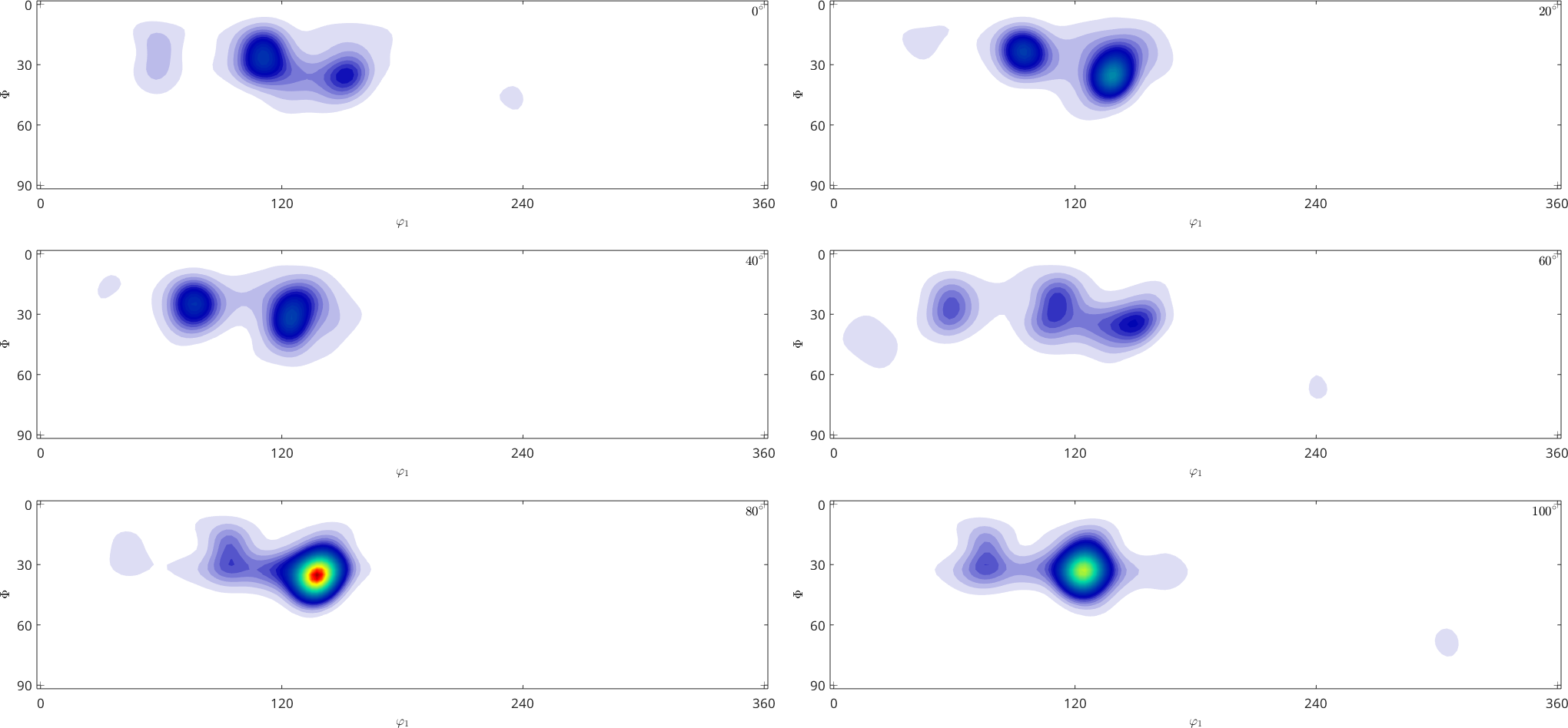
plot(F1)
ans =
0.0015
Furthermore, if the evaluation step is very expansive it might be a good idea to use the smaller Gauss-Legendre quadrature grid. The Gauss-Legendre quadrature lattice has half as many points as the default Clenshaw-Curtis quadrature lattice. But the quadrature method is much more time consuming.
% Compute the quadrature grid and weights
SO3G = quadratureSO3Grid(N,'GaussLegendre',SRight,SLeft);
% Evaluate your routine on that quadrature grid
tic
  v = odf.eval(SO3G);
toc
% and do quadrature
F2 = SO3FunHarmonic.quadrature(SO3G,v)

norm(F-F2)
Elapsed time is 3.165124 seconds.
F2 = SO3FunHarmonic (Quartz → xyz)
bandwidth: 50
weight: 1
ans =
0.0016