How to analyze slip transmission at grain boundaries
Import Titanium data
From Mercier D. - MTEX 2016 Workshop - TU Chemnitz (Germany) Calculation and plot on GBs of m' parameter Dataset from Mercier D. - cp-Ti (alpha phase - hcp)
mtexdata csl

% compute grains
[grains, ebsd.grainId] = calcGrains(ebsd('indexed'));

% make them a bit nicer
grains = smooth(grains);

% extract inner phase grain boundaries
gB = grains.boundary('indexed');

plot(ebsd,ebsd.orientations)
hold on
plot(grains.boundary)
hold off
ebsd = EBSD (y↑→x)
Phase Orientations Mineral Color Symmetry Crystal reference frame
0 5 (0.0032%) notIndexed
-1 154107 (100%) iron LightSkyBlue m-3m
Properties: ci, error, iq
Scan unit : um
X x Y x Z : [0, 511] x [0, 300] x [0, 0]
Normal vector: (0,0,1)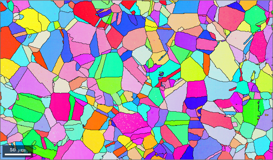
Taylor model
% consider Basal slip
sS = slipSystem.fcc(ebsd.CS)

% and all symmetrically equivalent variants
sS = sS.symmetrise;

% consider plane strain
q = 0.5;
eps = strainTensor(diag([-q 1 -(1-q)]));

% and compute Taylor factor as well as the active slip systems
[M,b,W] = calcTaylor(inv(grains.meanOrientation).*eps,sS);
sS = slipSystem (iron)
u v w | h k l CRSS
0 1 -1 1 1 1 1% find the maximum
[~,id] = max(b,[],2);The variable id contains now for each grain the id of the slip system with the largest Schmidt factor. In order to visualize it we first rotate for each grain the slip system with largest Schmid factor in specimen coordinates
sSGrain = grains.meanOrientation .* sS(id)

% and plot then the plane normal and the Burgers vectors into the centers
% of the grains

plot(grains,M)

largeGrains = grains(grains.numPixel > 10)

hold on
quiver(grains,sSGrain.trace,'displayName','slip plane trace')
hold on
quiver(grains,sSGrain.b,'displayName','slip direction','project2plane')
hold off

legend show
sSGrain = slipSystem (y↑→x)
CRSS: 1
size: 885 x 1
largeGrains = grain2d (y↑→x)
Phase Grains Pixels Mineral Symmetry Crystal reference frame
-1 442 153261 iron m-3m
boundary segments: 23334 (19528 µm)
inner boundary segments: 93 (82 µm)
triple points: 1444
Properties: meanRotation, GOS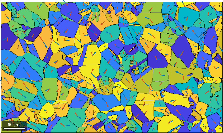
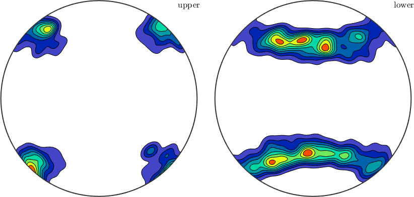
We may also analyze the distribution of the slip directions in a pole figure plot
plot(sSGrain.b)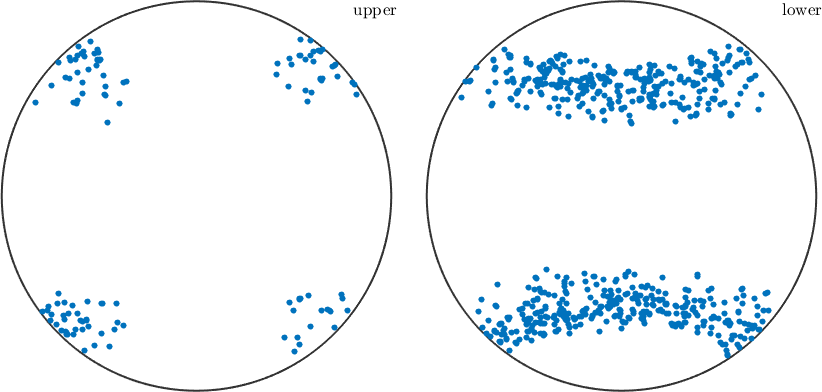
The same as a contour plot. We see a clear trend towards east.
plot(sSGrain.b,'contourf')