Specimen Directions (The Class vector3d)
This section describes the class vector3d and gives an overview how to deal with specimen directions in MTEX.
Class Description
Specimen directions are three-dimensional vectors in the Euclidean space represented by coordinates with respect to an outer specimen coordinate system x, y, z. In MTEX Specimen directions are represented by variables of the class vector3d.
Defining Specimen Directions
The standard way to define a specimen directions is by its coordinates.
v = vector3d(1,1,0);
This gives a single vector with coordinates (1,1,0) with respect to the x, y , z coordinate system. A second way to define a specimen directions is by its spherical coordinates, i.e. by its polar angle and its azimuth angle. This is done by the option polar.
polar_angle = 60*degree;
azimuth_angle = 45*degree;
v = vector3d.byPolar(polar_angle,azimuth_angle);
Finally, one can also define a vector as a linear combination of the predefined vectors xvector, yvector, and zvector
v = xvector + 2*yvector;
Calculating with Specimen Directions
As we have seen in the last example. One can calculate with specimen directions as with ordinary number. Moreover, all basic vector operation as "+", "-", "*", inner product, cross product are implemented.
u = dot(v,xvector) * yvector + 2 * cross(v,zvector);
Using the brackets v = [v1,v2] two specimen directions can be concatened. Now each single vector is accesable via v(1) and v(2).
w = [v,u];
w(1)
w(2)
ans = vector3d
 size: 1 x 1
  x y z
  1 2 0

ans = vector3d
 size: 1 x 1
  x  y  z
  4 -1  0
When calculating with concatenated specimen directions all operations are performed componentwise for each specimen direction.
w = w + v;
Besides the standard linear algebra operations, there are also the following functions available in MTEX.
angle(v1,v2) % angle between two specimen  directions
dot(v1,v2)   % inner product
cross(v1,v2) % cross product
norm(v)      % length of the specimen directions
sum(v)       % sum over all specimen directions in v
mean(v)      % mean over all specimen directions in v
polar(v)     % conversion to spherical coordinates
% A simple example for applying the norm function is to normalize a set of
% specimen directions

w = w ./ norm(w)
w = vector3d
 size: 1 x 2
         x        y        z
  0.447214 0.894427        0
  0.980581 0.196116        0
Plotting three dimensionl vectors
The plot function allows you to visualize an arbitrary number of specimen directions in a spherical projection
plot([zvector,xvector+yvector+zvector],'labeled')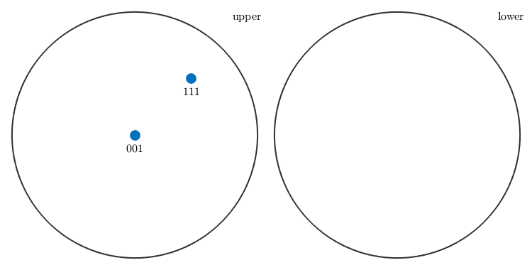
random vectors
equispaced grids
regular grids
alginment of the plot
Complete Function list
| Syntax | |
| v = vector3d(x,y,z) | |
| v = vector3d(x,y,z,'antipodal') | |
| v = vector3d('polar',theta,rho) | |
| Input | |
| x,y,z | cart. coordinates |
| Flags | |
| antipodal | consider vector as an axis and not as an direction |
| See also | |
| AxialDirectional |
| DocHelp 0.1 beta |