Slip Transmission
How to analyze slip transmission at grain boundaries
| On this page ... |
| Import Titanium data |
| Schmid Factor |
| Resolved shear stress |
| Compatibility of slip systems |
| Plot m' in misorientation space |
Import Titanium data
From Mercier D. - MTEX 2016 Workshop - TU Chemnitz (Germany) Calculation and plot on GBs of m' parameter Dataset from Mercier D. - cp-Ti (alpha phase - hcp)
mtexdata titanium

% compute grains
[grains, ebsd.grainId] = calcGrains(ebsd('indexed'));

% make them a bit nicer
grains = smooth(grains);

% extract inner phase grain boundaries
gB = grains.boundary('indexed');

plot(ebsd,ebsd.orientations)
hold on
plot(grains.boundary)
hold off
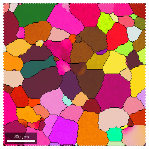
Schmid Factor
% consider Basal slip
sSBasal = slipSystem.basal(ebsd.CS)

% and all symmetrically equivalent variants
sSBasal = sSBasal.symmetrise;

% compute Schmid factor for all slip systems
SF = sSBasal.SchmidFactor(inv(grains.meanOrientation) * xvector);

% find the maximum Schmidt factor
[SF,id] = max(SF,[],2);

% and plot it for each grain
plot(grains,SF)
mtexColorbar
sSBasal = slipSystem
 mineral: Titanium (Alpha) (622, X||a, Y||b*, Z||c)
 size: 1 x 1
  U    V    T    W  | H    K    I    L CRSS
  1    1   -2    0    0    0    0    1    1
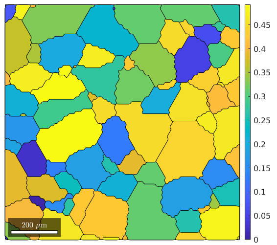
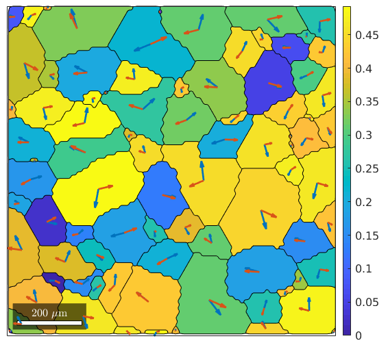
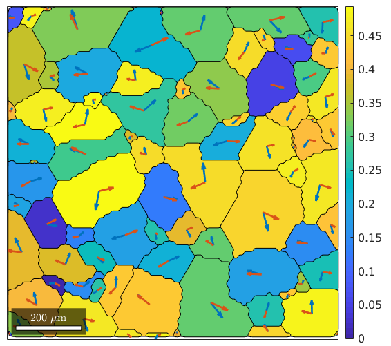
The variable id contains now for each grain the id of the slip system with the largest Schmidt factor. In order to visualize it, we first rotate for each grain the slip system with largest Schmid factor in specimen coordinates
sSGrain = grains.meanOrientation .* sSBasal(id)

% and then plot the plane normal and the Burgers vectors into the centers
% of the grains

hold on
quiver(grains,cross(sSGrain.n,zvector),'displayName','slip plane')
hold on
quiver(grains,sSGrain.b,'displayName','slip direction')
hold off
sSGrain = slipSystem
 CRSS: 1
 size: 85 x 1
We may also analyse the distribution of the slip directions in a pole figure plot
plot(sSGrain.b)
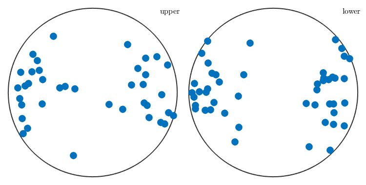
The same as a contour plot. We see a clear trend towards the east.
plot(sSGrain.b,'contourf')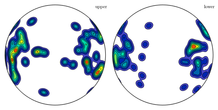
Resolved shear stress
We could do the same as above with a more general stress tensor. However, the result is a bit different. TODO: why the directions do not point towards east???
% more general syntax for the same stress tensor
sigma = stressTensor.uniaxial(xvector);

% compute Schmid factor for all slip systems
SF = sSBasal.SchmidFactor(inv(grains.meanOrientation) * sigma);

% find the maximum Schmidt factor
[SF,id] = max(SF,[],2);

% plot the Schmid factor
plot(grains,SF)
mtexColorbar

% active slip system in specimen coordinates
sSGrain = grains.meanOrientation .* sSBasal(id)

% and plot then the plance normal and the Burgers vectors into the centers
% of the grains
hold on
quiver(grains,cross(sSGrain.n,zvector),'displayName','slip plane')
hold on
quiver(grains,sSGrain.b,'displayName','slip direction')
hold off
sSGrain = slipSystem
 CRSS: 1
 size: 85 x 1
Compatibility of slip systems
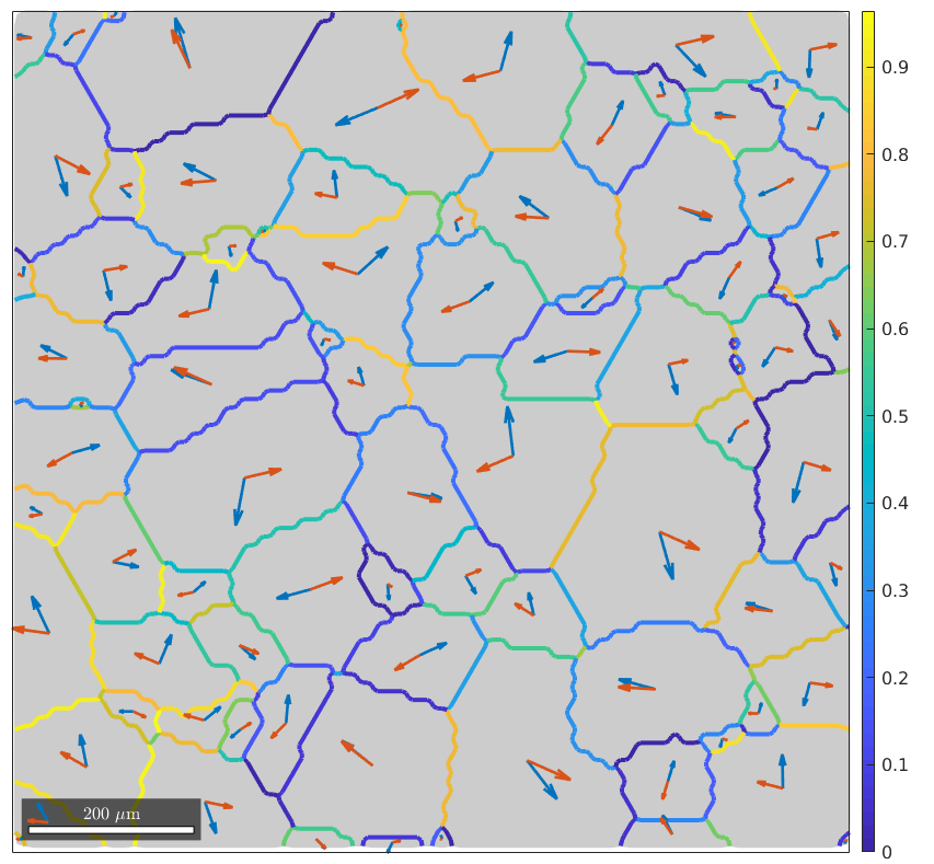
Next, we want to analyze, how much geometrically compatible the slip systems with highest Schmid factor are at the grain boundaries
% some background
plot(grains,'FaceColor',0.8*[1 1 1],'figSize','large')

% compute m'
id = gB.grainId;
mP = mPrime(sSGrain(id(:,1)),sSGrain(id(:,2)));

% plot m' along the grain boundaries
hold on
plot(gB,mP,'linewidth',3)
mtexColorbar

% and plot then the plance normal and the Burgers vectors into the centers
% of the grains
hold on
quiver(grains,cross(sSGrain.n,zvector),'displayName','slip plane')
hold on
quiver(grains,sSGrain.b,'displayName','slip direction')
hold off
Plot m' in misorientation space
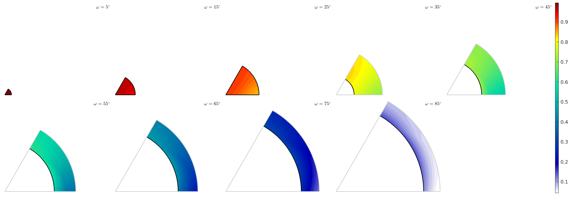
Since m' depends on the misorientation only why may plot it directly in misorientation space
% set up an axis angle plot
sP = axisAngleSections(sSBasal.CS,sSBasal.CS);

% generate a grid of misorientations
moriGrid = sP.makeGrid;

% compute mPrime for all misorientations
sSBasal = slipSystem.basal(ebsd.CS);
mP = max(mPrime(sSBasal,moriGrid*sSBasal.symmetrise),[],2);

% plot mPrime
sP.plot(mP,'smooth')
mtexColorbar
| DocHelp 0.1 beta |