Model ODFs
Describes how to define model ODFs in MTEX, i.e., uniform ODFs, unimodal ODFs, fibre ODFs, Bingham ODFs and ODFs defined by its Fourier coefficients.
| On this page ... |
| Introduction |
| The Uniform ODF |
| Unimodal ODFs |
| Fibre ODFs |
| ODFs given by Fourier coefficients |
| Bingham ODFs |
| Combining model ODFs |
Introduction
MTEX provides a very simple way to define model ODFs. Generally, there are five types to describe an ODF in MTEX:
- uniform ODF
- unimodal ODF
- fibre ODF
- Bingham ODF
- Fourier ODF
The central idea is that MTEX allows you to calculate mixture models, by adding and subtracting arbitrary ODFs. Model ODFs may be used as references for ODFs estimated from pole figure data or EBSD data and are instrumental for pole figure simulations and single orientation simulations.
The Uniform ODF
The most simplest case of a model ODF is the uniform ODF
which is everywhere identical to one. In order to define a uniform ODF one needs only to specify its crystal and specimen symmetry and to use the command uniformODF.
cs = crystalSymmetry('cubic');
ss = specimenSymmetry('orthorhombic');
odf = uniformODF(cs,ss)
odf = ODF
  crystal symmetry : m-3m
  specimen symmetry: mmm

  Uniform portion:
    weight: 1
Unimodal ODFs
An unimodal ODF

is specified by a radially symmetrial function  centered at a modal orientation,
  and. In order to define a unimodal ODF one needs
- a preferred orientation mod1
- a kernel function psi defining the shape
- the crystal and specimen symmetry
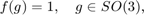
ori = orientation.byMiller([1,2,2],[2,2,1],cs,ss);
psi = vonMisesFisherKernel('HALFWIDTH',10*degree);
odf = unimodalODF(ori,psi)

plotPDF(odf,[Miller(1,0,0,cs),Miller(1,1,0,cs)],'antipodal')
odf = ODF
  crystal symmetry : m-3m
  specimen symmetry: mmm

  Radially symmetric portion:
    kernel: van Mises Fisher, halfwidth 10°
    center: (297°,48°,27°)
    weight: 1
For simplicity one can also omit the kernel function. In this case the default de la Vallee Poussin kernel is chosen with half width of 10 degree.
Fibre ODFs
A fibre is represented in MTEX by a variable of type fibre.
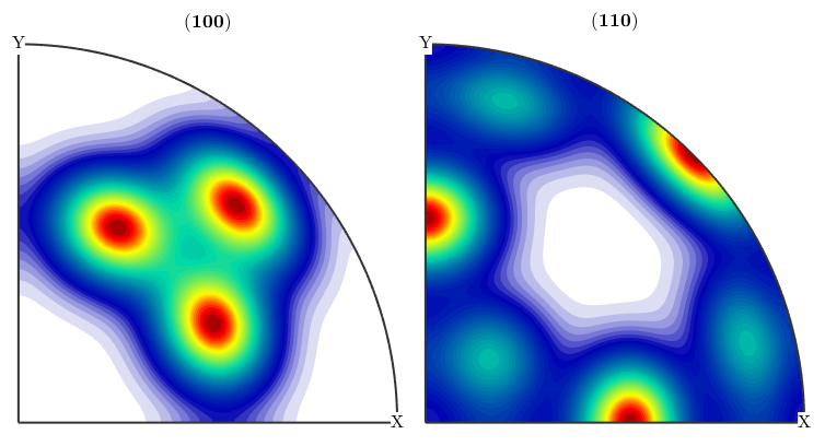
% define the fibre to be the beta fibre
f = fibre.beta(cs)

% define a fibre ODF
odf = fibreODF(f,ss,psi)

% plot the odf in 3d
plot3d(odf)
f = fibre
 size: 1 x 1
 crystal symmetry:  m-3m
 o1: (180°,35°,45°)
 o2: (270°,63°,45°)

odf = ODF
  crystal symmetry : m-3m
  specimen symmetry: 1

  Fibre symmetric portion:
    kernel: van Mises Fisher, halfwidth 10°
    fibre: (---) - -0.23141,-0.23141,0.94494
    weight: 1
ODFs given by Fourier coefficients
In order to define a ODF by it Fourier coefficients the Fourier coefficients C has to be given as a literally ordered, complex valued vector of the form

where  denotes the order of the Fourier coefficients.
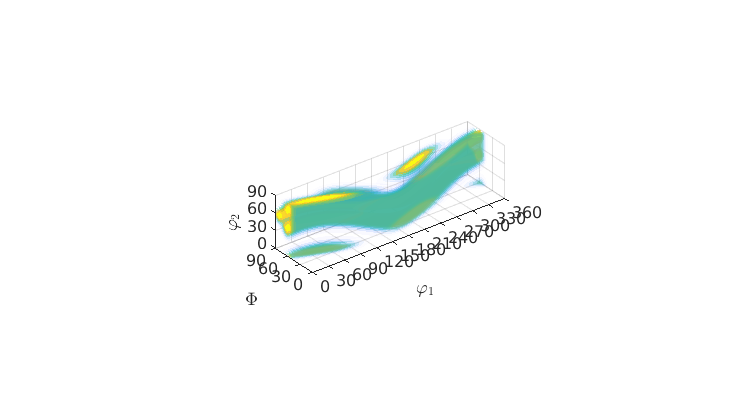
cs   = crystalSymmetry('1');    % crystal symmetry
C = [1;reshape(eye(3),[],1);reshape(eye(5),[],1)]; % Fourier coefficients
odf = FourierODF(C,cs)

plot(odf,'sections',6,'silent','sigma')
mtexColorMap LaboTeX
odf = ODF
  crystal symmetry : 1, X||a, Y||b*, Z||c*
  specimen symmetry: 1
  antipodal:         true

  Harmonic portion:
    degree: 2
    weight: 1
plotPDF(odf,[Miller(1,0,0,cs),Miller(1,1,0,cs)],'antipodal')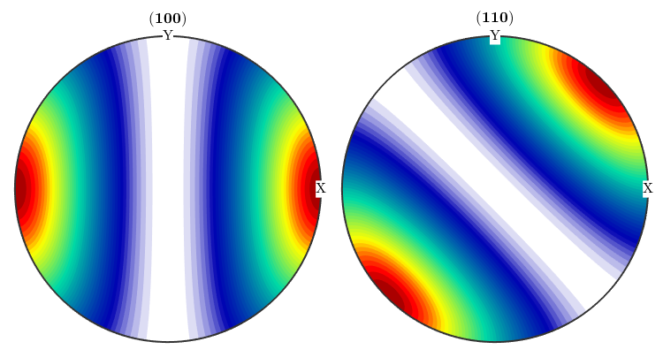
Bingham ODFs
The Bingham quaternion distribution
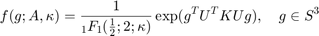
has a (4x4)-orthogonal matrix  and shape parameters
  as argument. The (4x4) matrix can be interpreted as 4 orthogonal quaternions
  , where the
  allow different shapes, e.g.
- unimodal ODFs
- fibre ODF
- spherical ODFs
A Bingham distribution is characterized by
- four orientations
- four values lambda
cs = crystalSymmetry('-3m');Bingham unimodal ODF
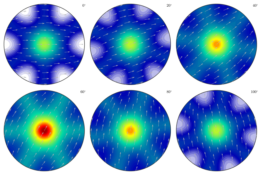
% a modal orientation
mod = orientation.byEuler(45*degree,0*degree,0*degree);

% the corresponding Bingham ODF
odf = BinghamODF(20,mod,cs)

plot(odf,'sections',6,'silent','contourf','sigma')
odf = ODF
  crystal symmetry : -3m1, X||a*, Y||b, Z||c*
  specimen symmetry: 1

  Bingham portion:
     kappa: 20 0 0 0
    weight: 1
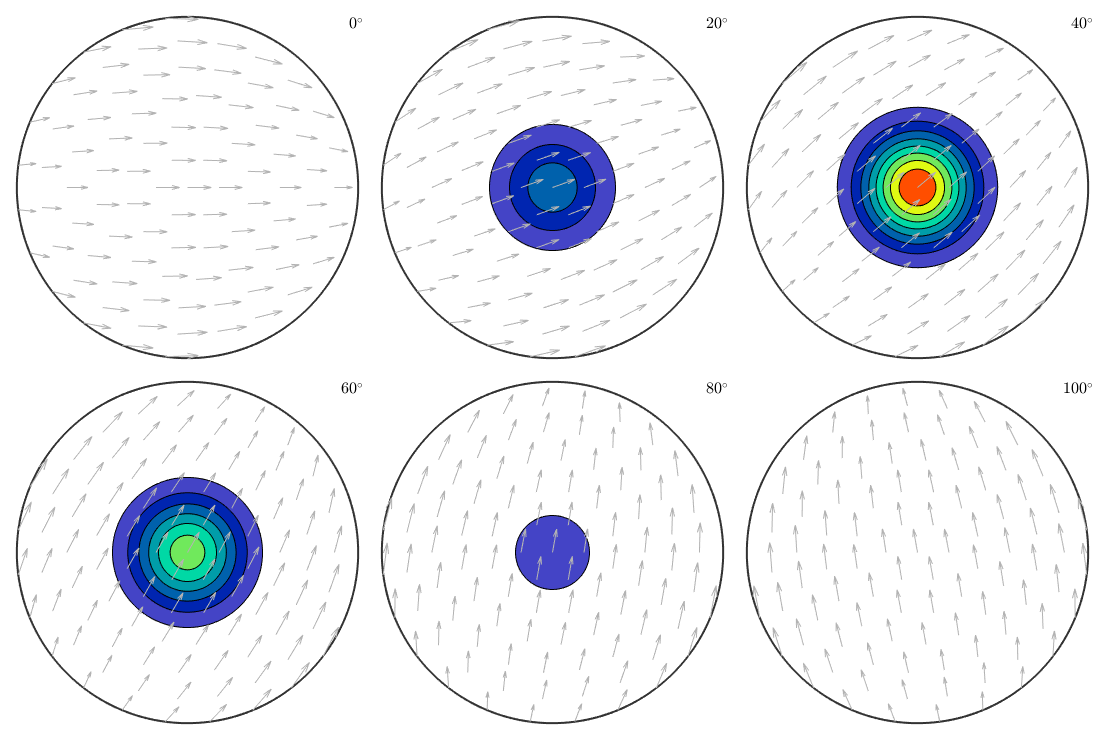
Bingham fibre ODF
odf = BinghamODF([-10,-10,10,10],quaternion(eye(4)),cs)

plot(odf,'sections',6,'silent','sigma')
odf = ODF
  crystal symmetry : -3m1, X||a*, Y||b, Z||c*
  specimen symmetry: 1

  Bingham portion:
     kappa: -10 -10 10 10
    weight: 1
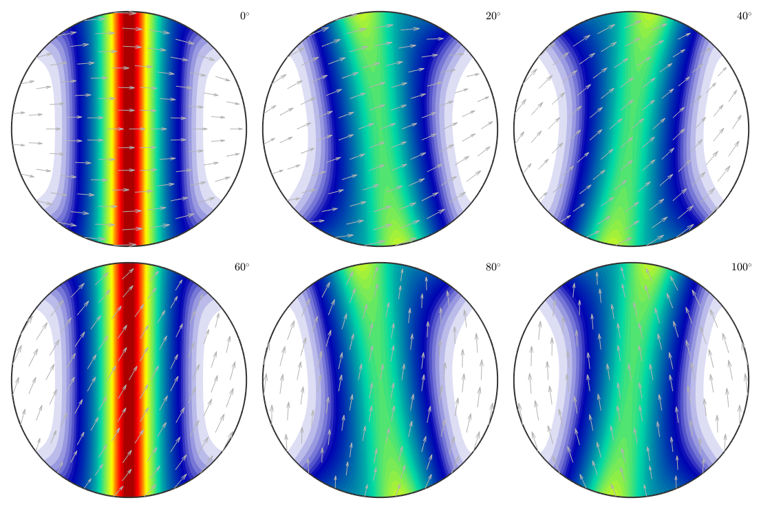
Bingham spherical ODF
odf = BinghamODF([-10,10,10,10],quaternion(eye(4)),cs)

plot(odf,'sections',6,'silent','sigma');
odf = ODF
  crystal symmetry : -3m1, X||a*, Y||b, Z||c*
  specimen symmetry: 1

  Bingham portion:
     kappa: -10 10 10 10
    weight: 1
Combining model ODFs
All the above can be arbitrarily rotated and combined. For instance, the classical Santafe example can be defined by commands
cs = crystalSymmetry('cubic');
ss = specimenSymmetry('orthorhombic');

psi = vonMisesFisherKernel('halfwidth',10*degree);
mod1 = orientation.byMiller([1,2,2],[2,2,1],cs,ss);

odf =  0.73 * uniformODF(cs,ss) + 0.27 * unimodalODF(mod1,psi)

close all
plotPDF(odf,[Miller(1,0,0,cs),Miller(1,1,0,cs)],'antipodal')
odf = ODF
  crystal symmetry : m-3m
  specimen symmetry: mmm

  Uniform portion:
    weight: 0.73

  Radially symmetric portion:
    kernel: van Mises Fisher, halfwidth 10°
    center: (297°,48°,27°)
    weight: 0.27

| DocHelp 0.1 beta |